Random Walks in Higher Dimensions

So I was thinking about the dynamics of training, and looking for a way to model some phenomenon I had observed.

Initially, I had dismissed Brownian motion/random walk as an option because the trend was clearly linear — not square root. But then I was asked what Brownian motion looked like in higher dimensions and I panicked.

I had assumed that Brownian motion was universal — that dimensionality didn't enter into the equation (for average distance from the origin as a function of time). But now I was doubting myself.

So I did a quick derivation, which I'm sharing because it gave me a new way to interpret the chi-squared distribution. Here's the set-up: we have a walker on a $D$-dimensional (square) lattice. At every timestep, the walker chooses uniformly among the $2D$ available directions to take one step.

This means that every dimension is sampled on average once every $D$ timesteps, so we can treat a $D$-dimensional walker after $N$ timesteps as a collection of $D$ independent $1$-dimensional walkers after $N/D$ timesteps.

If the $1$-dimensional walker's probability distribution is just a Gaussian centered at $0$ with standard deviation $\sqrt N$, then the probability for the $D$-dimensional walker is the product of $D$ univariate gaussians centered at $0$ with standard deviation $\sqrt{{N}/{D}}$.

But that means that the expected distance traveled by the $D$-dimensional walker, $\sqrt{\mathbb E[|\vec X|^2]}$, is just the square root of the chi-squared distribution,

scaled by a factor $\sqrt{N/D}$. (This is not the chi distribution, which we'd want if we were taking the square root before the expectation.)

In this context, $D$ is the number of degrees of freedom. After multiplying the mean of the chi distribution by our factor $\sqrt{N/D}$, we get

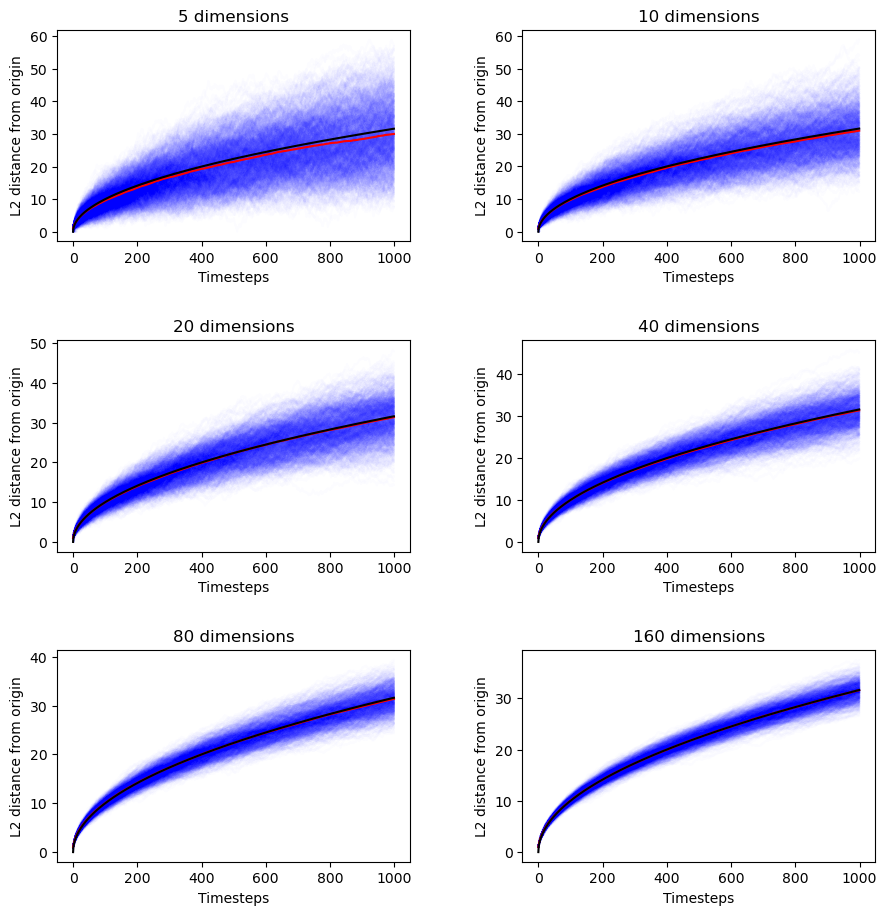
It's independent of lattice dimensionality. Just as I originally thought before starting to doubt myself before going down this rabbit hole before reestablishing my confidence.

If that's not enough for you, here are the empirical results.

def random_hyperwalk(n_dims: int, n_samples: int = 1_000, n_timesteps: int = 10_000) -> np.ndarray:
    state = np.zeros((n_samples, n_dims))
    distances = np.zeros((n_samples, n_timesteps))

    for t in tqdm(range(n_timesteps)):
        step = np.random.choice(np.arange(n_dims), n_samples)
        # print(step)
        directions = np.random.choice([-1, 1], n_samples)
        # print(directions)

        # TODO: vectorize this
        for i in range(n_samples):
            state[i, step[i]] += directions[i]

        # print(step, directions, state[:, step])
        distances[:, t] = np.linalg.norm(state, axis=1)

    return distances

def random_hyperwalk_scaling(n_dim_range: List[int], n_samples: int = 1_000, n_timesteps: int = 10_000):
    timesteps = np.arange(n_timesteps)
    predictions = np.sqrt(timesteps)
    trajectories = np.zeros((len(n_dim_range), n_samples, n_timesteps))

    fig, ax = plt.subplots(len(n_dim_range) // 2, 2, figsize=(10, 10))
    fig.tight_layout(pad=5.0)

    for I, n_dims in enumerate(n_dim_range):
        i, j = I // 2, I % 2

        trajectories[I, :, :] = random_hyperwalk(n_dims, n_samples, n_timesteps)
        mean_distances = np.mean(trajectories[I, :, :], axis=0)

        for k in range(n_samples):
            ax[i][j].plot(timesteps, trajectories[I, k, :], color="blue", alpha=0.01)
    
        ax[i][j].set_title(f"{n_dims} dimensions")
        ax[i][j].plot(timesteps, mean_distances, color="red")
        ax[i][j].plot(timesteps, predictions, color="black")
        ax[i][j].set_xlabel("Timesteps")
        ax[i][j].set_ylabel("L2 distance from origin")

    plt.show()


random_hyperwalk_scaling([5, 10, 20, 40, 80, 160], n_samples=1000, n_timesteps=1000)