Scaling Laws of Path dependence

NOTE: Work in Progress

How much do the models we train depend on the path they follow through weight space?

Should we expect to always get the same models for a given choice of hyperparameters and dataset? Or do the outcomes depend highly on quirks of the training process, such as the weight initialization and batch schedule?

If models are highly path-dependent, it could make alignment harder: we'd have to keep a closer eye on our models during training for chance forays into deception. Or it could make alignment easier: if alignment is unlikely by default, then increasing the variance in outcomes increases our odds of success.

Vivek Hebbar and Evan Hubinger have already explored the implications of path-dependence for alignment here. In this post, I'd like to formalize "path-dependence" in the language of dynamical systems, and share the results of experiments inspired by this framing.

From these experiments, we find novel scaling laws relating choices of hyperparameters like model size, learning rate, and momentum to the trajectories of these models during training. We find functional forms that provide a good empirical fit to these trajectories across a wide range of hyperparameter choices, datasets, and architectures.

Finally, we study a set of toy models that match the observed scaling laws, which gives us insight into the possible mechanistic origins of these trends, and a direction towards building a theory of the dynamics of training.

Formalizing Path-dependence

Hebbar and Hubinger define path-dependence "as the sensitivity of a model's behavior to the details of the training process and training dynamics." Let's make that definition more precise. To start, let us formalize the learning process as a dynamical system over weight space.

In the context of machine learning, our goal is (usually) to model some "true" function $f^* : \mathcal X \to \mathcal Y$¹. To do this, we construct a neural network, $f: \mathcal X \times \mathcal W \to \mathcal Y$, which induces a model of $f^*$ upon fixing a choice of weights, $w \in \mathcal W \subset \mathbb R^D$. For convenience, we'll denote the resulting model with a subscript, i.e., $\mathcal F \ni f_{w}(x):= f(x, w)$.²

To find the weights, $w_\mathrm{opt}$, such that $f_\text{opt} := f_{w_\text{opt}}$ is as "close" as possible to $f^*$, we specify a loss function $L_n$, which maps a choice of parameters and a set of training examples, $\mathbf d_\text{train} = \{(x_{i},y_i)\}_{i=1}^n \in \mathcal Z^n$, to a scalar "loss"³:

For a fixed choice of dataset, we denote the empirical loss, $L_\text{train}(w) =L(w, \mathbf d_\text{train})$. Analogously, we can define a test loss, $L_\text{test}$ over a corresponding test set, and batch loss, $L^{(t)}_\mathbf{b}(w)$, for a batch $\mathbf b^{(t)} \subset \mathbf d_\text{train}$.

Next, we choose an optimizer, $\Phi$, which iteratively updates the weights (according to some variant of SGD),

The optimizer depends on some hyperparameters, $h \in \mathcal H$, and learning schedule $\mathbf b = \{\mathbf b^{(t)}\}_{t=1}^T$ of $T$ batches, $\mathbf b^{(t)} \in \boldsymbol{\mathcal B}$. Note: this learning schedule covers all $N_\text{epochs}$ epochs. In other words, if an epoch consists of $T_\text{epochs}$ batches, then $T/ T_\text{epochs} = N_\text{epochs}$. Within any given epoch, the batches are disjoint, but across epochs, repetition is allowed (though typically no batch will be repeated sample for sample).

If we take the learning schedule and hyperparameters as constant, we obtain a discrete-time dynamical system over parameter space, which we denote $\Phi_{\mathbf b, h}: \mathcal W \to \mathcal W$.

Two Kinds of Path Dependence

Given this dynamical system, $\Phi_{\mathbf b, h}$ over weight space, let us contrast two kinds of path dependence:

1. Global path dependence. Given some distribution over starting weights, $p(w^{(0)})$, hyperparameters, $p(h)$, or batches, $p(\mathbf b)$, what is the resulting distribution over final weights, $p(w^{(T)})$?
2. Local path dependence. For some choice of initial weights, $w^{0}$, hyperparameters, $h$, or batches, $\mathbf b$, and a small perturbation (of size $\epsilon \ll 1$) to one of these values, how "different" does the perturbed model end up being from the baseline unperturbed model? In the limit of infinitesimal perturbations, this reduces to computing derivatives of the kind $\frac{\partial w^{(T)}}{\partial{w^{(0)}}}$, $\frac{\partial w^{(T)}}{\partial{h}}$, and $\frac{\partial w^{(T)}}{\partial{b^{(t)}}}$.

Though we ultimately want to form global statements of path dependence, the distributions involved are generally intractable (which require us to resort to empirical approximations). In the local view, we rarely care about specific perturbations, so we end up studying the relation between a similarly intractable distribution over perturbations $p(\delta)$ and $p(w^{(T)})$. Still, this is much easier to explore empirically because of its smaller support.

Continuous vs. Discrete Hyperparameters

Below, is a table of the various hyperparameters we encounter in our model, weight initializer, optimizer, and dataloader. Here, we're taking "hyperparameter" in the broadest sense to incorporate even the dataset and choice of model architecture.

To study local perturbations, we're interested in those hyperparameters that we can vary continuously. E.g.: we can gradually increase the magnitude $\epsilon$ of the perturbation applied to our baseline model, as well as the momenta, regularization coefficients, and learning rates of the optimizer, but we can't smoothly vary the number of layers in our model or the type of optimizer we're using.

From weights to functions

The problem with studying dynamics over $\mathcal W$ is that we don't actually care about $w \in \mathcal W$. Instead, we care about the evolution in function space, $\mathcal F$, which results from the mapping $m: \mathcal W \ni w \mapsto f_{w}\in \mathcal F$.

We care about this evolution because the mapping to function space is non-injective; the internal symmetries of $m$ ensure that different choices of $w\in \mathcal W$ can map to the same function $f \in \mathcal F$.[1] As a result, distance in $\mathcal W$ can be misleading as to the similarity of the resulting function.

The difficulty with function space is that it is infinite-dimensional, so studying it is that much more intractable than studying weight space. In practice, then, we have to estimate where we are in function space over a finite number of samples of input-output pairs, for which we typically use the training and test sets.

However, even though we have full knowledge of $\mathcal W$, we can't resolve exactly where we are in $\mathcal F$ from any finite set of samples. At best, we can resolve the level set in $\mathcal F$ with a certain empirical performance (like training/test loss). This means our sampling procedure acts as a second kind of non-injective map from $\mathcal F\to \mathcal F_\text{obs} = (\mathcal X \times \mathcal Y)^n$.

A note on optimizer state: If we want to be exhaustive, let us recall that optimizers might have some internal state, $s \in \mathcal S$. E.g., for Adam, $s_{t}= (m_t, v_t)$, a running average of the first moment and second moment of the gradients, respectively. Then, the dynamical system over $\mathcal W$ is more appropriately a dynamical system over the joint space $\mathcal W \times \mathcal S$. Completing this extension will have to wait for another day; we'll ignore it for now for the sake of simplicity and because, in any case, $s_t$, tends to be a deterministic function of $\mathbf b$ and $h$.

Experiments

In section XX, we defined path dependence as about understanding the relation between $(P(B_t), P(W_0), P(H))$ and $(P(W_{T}), P(F_{T}))$. As mentioned, there are two major challenges:

1. In general, we have to estimate these distributions empirically, and training neural networks is already computationally expensive, so we're restricted to studying smaller networks and datasets.
2. The mapping $m:\mathcal W\to \mathcal F$ is non-straightforward because of the symmetries of $m$.

To make it easier for ourselves, let us restrict our attention to the narrower case of studying local path-dependence.

a (small) perturbation, $\epsilon$, to one of $(b_{t}, w_{0}, h)$. E.g., we'll study probability densities of the kind $p(\mathbf w_0)=\mathcal N(\mathbf w_{0}|\mathbf w_\text{baseline}, \epsilon \mathbf 1)$. For discrete variables (like the number of layers, network width, and batch schedule), there's a minimum size we can make $\epsilon$,

Within dynamical systems theory, there are two main ways to view dynamical systems:

1. The trajectory view studies the evolution of points like $(w_0, w_1, \dots, w_T)$ and $(f_1, f_2, \dots, f_T)$.
2. The probability view studies the evolution of densities like $(p_0(w), p_1(w), \dots, p_T(w))$ and $(p_1(f), p_2(f), \dots, p_T(f))$.

Both have something to tell us about path dependence:

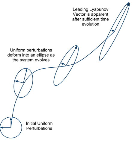
1. In the trajectory view, sensitivity of outcomes becomes a question of calculating Lyapunov exponents, the rate at which nearby trajectories diverge/converge.
2. In the probability view, sensitivity of outcomes becomes a question of measuring autocorrelations, $\langle w_{i} w_{i+\tau}\rangle$ and $\langle f_{i} f_{i+\tau} \rangle$.

Tracking Trajectories

The experimental set-up involves taking some baseline model, $m_0$, then applying a Gaussian perturbation to the initial weights with norm $\epsilon$, to obtain a set of perturbed models $\{m_i\} _{i=1}^{n _\text{models}}$. We train these models on MNIST (using identical batch schedules for each model).

Over the course of training, we track how these models diverge via several metrics (see next subsection). For each of these, we study how the rate of divergence varies for different choices of hyperparameters: momentum $\beta$, weight decay $\lambda$, learning rate $\eta$, hidden layer width (for one-hidden-layer models), and number of hidden layers. Moving on from vanilla SGD, we compare adaptive variants like Adam and RMSProp.

TODO: Non-FC models. Actually calculate the rate of divergence (for the short exponential period at the start). Perform these experiments for several different batch schedules. Perturbations in batch schedule. Other optimizers besides vanilla SGD.

Measuring distance

• $d_\mathbf{w}^{(p)}(m_i, m_0)$: the $p$-norm between the weight vectors of each perturbed model and the baseline model. We'll ignore the $p$ throughout and restrict to the case $p=2$. This is the most straightforward notion of distance, but it's flawed in that it can be a weak proxy for distance in $\mathcal F$ because of the internal symmetries of the model.
• $\frac{d_{\mathbf w}(m_{i}, m_0)}{|\mathbf w_{0}|}$: the relative $p$-norm between weight vectors of each perturbed model.
• $L_\text{train,test}(m_i)$: the training/test losses
• $\delta L_\text{train, test}(m_{i}, m_0)$: the training/test loss relative (difference) to the baseline model $m_0$
• $f_\text{train, test}(m_i)$, $\delta f_\text{train, test}(m_i, m_0)$: the training/test set classification accuracy and relative classification accuracy.
• $L_\text{train cf., test cf.}$ and $f_\text{train cf., test cf.}$: same as above, but we take the predictions of the baseline model as the ground truth (rather than the actual labels in the test set).

A few more metrics to include:

• $d^\text{perm.}_{\mathbf w}$: the l2 norm after adjusting for permutation differences (as described in Ainsworth et al.)
• $\int_{\mathbf w_0}^{\mathbf w_{i}^\text{perm.}} L_\text{train (cf.), test (cf.)}(\mathbf w) d\mathbf w$. The loss integrated over the linear interpolation between two models' weights after correcting for permutations (as described in Ainsworth et al.)

Tracking Densities

TODO

Results

One-hidden-layer Models

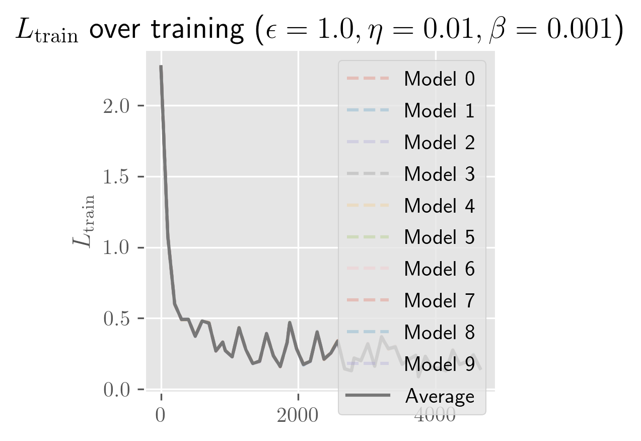
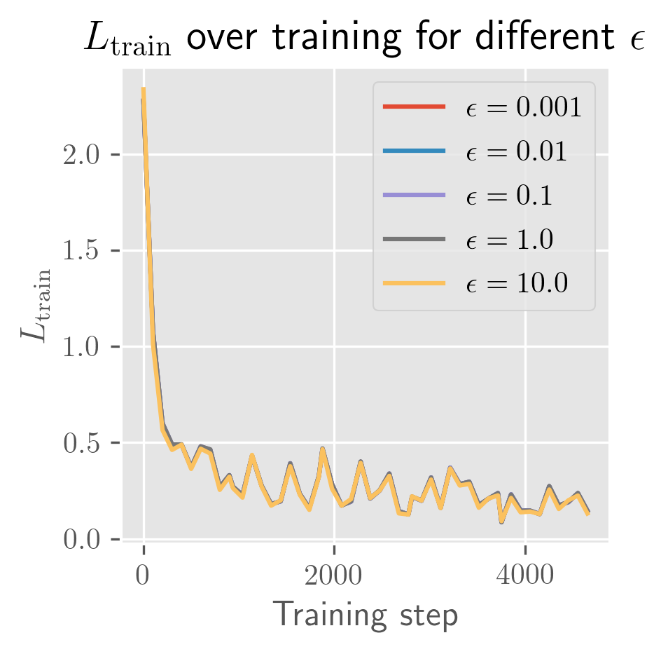
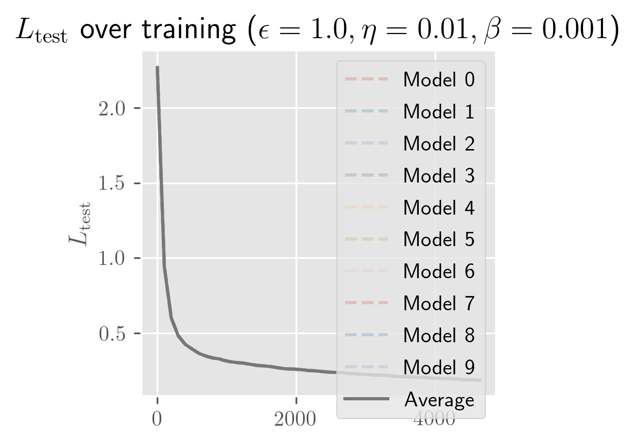
What's remarkable about one-hidden-layer models is how little the model depends on weight initialization: almost all of the variance seems to be explained by the batch schedule. Even for initial perturbations of size $\epsilon=10$¹, the models appear to become almost entirely equivalent in function space across the entire training process. In the figure below, you can see that the differences in $L_\text{train}$ are imperceptible (both for a fixed $\epsilon$ and across averages over different $\epsilon$).

TODO: I haven't checked $\epsilon/|\mathbf w|$. I'm assuming this is >1 for $\epsilon=10$ (which is why I find this surprising), but I might be confused about PyTorch's default weight initialization scheme. So take this all with some caution.

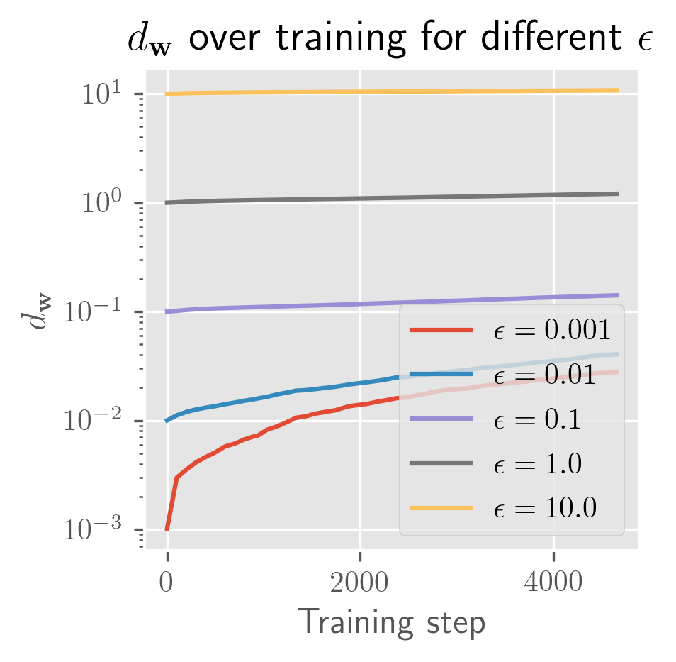
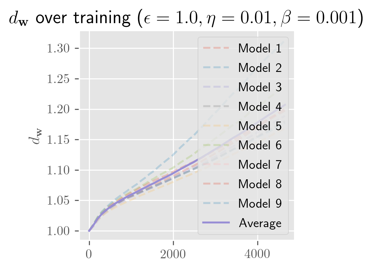
The rate of growth for $d_\mathbf{w}$ has a very short exponential period (shorter than a single epoch), followed by a long linear period (up to 25 epochs, long past when the error has stabilized). In some cases, you'll see a slight bend upwards or downwards. I need more time to test over more perturbations (right now it's 10 perturbed models) to clean this up. Maybe these trends change over longer periods, and with a bit more time I'll test longer training runs and over more perturbations.

Hyperparameters

• Momentum: ($\beta=0.1, 0.5, 0.9$) The $d_\textbf w$ curves look slightly more curved upwards/exponential but maybe that's confirmation bias (I expect momentum to make divergence more exponential back when I expected exponential divergence). Small amounts of momentum appear to increase convergence (relative to other models equivalent up to momentum), while large amounts increase divergence (towards . For very small amounts, the effect appears to be negligible. Prediction: the $d_w$ curves curve down because in flat basins, momentum slows you down.
• Learning rate: Same for $\eta=10^{-3}, 10^{-2}, 10^{-1}$. (Not too surprising) TODO: Compare directly between different learning rates. Can we see $\eta$ back in the slope of divergence? Prediction: This should not make much of a difference. I expect that correcting for the learning rate should give nearly identical separation slopes.
• Weight Decay: TODO for $\lambda=10^{-3}, 10^{-2}, 10^{-1}$. Prediction: $d_w$ will shrink (because $|w|$ will shrink). The normalized $d_w/|w|$ will curve downwards because we break the ReLU-scaling symmetry which means the volume of our basins will shrink
• Width: TODO. Both this and depth require care. With different sizes of $\mathbf w$, we can't naively compare norms. Is it enough to divide by $\dim \mathbf w$? Prediction: I expect the slope of divergence to increase linearly with the width of a one-layer network (from modeling each connection as separating of its own linear accord).
• Depth: TODO. Prediction: I expect the shape of $d_w$ for each individual layer to become more and more exponential with depth (because the change will be the product of layers that diverge linearly independently). I expect this to dominate the overall divergence of the networks.
• Architecture: Prediction: I expect convolutional architectures to decrease the rate of separation (after correcting for the number of parameters).
• Optimizer:
  • Prediction: I expect adaptive techniques to make the rate of divergence exponential.

Datasets

• Computer Vision
  • MNIST
  • Fashion-MNIST
  • Imagenet: Prediction: I expect Imagenet to lead to the same observations as MNIST (after correcting for model parameter count).
• Natural Language
  • IMDb movie review database

Why Linear?

I'm not sure. My hunch going in was that I'd see either exponential divergence (indicating chaos) or square root divergence (i.e., Brownian noise). Linear surprises me, and I don't yet know what to make of it.

Maybe all of this is just a fact about one-hidden-layer networks. If each hidden layer evolves independently linearly, maybe this combines additively into something Brownian. Or maybe it's multiplicative (so exponential).

Deep Models

TODO

Appendix

Weight Initialization

For ReLU-based networks, we use a modified version of Kaiming (normal) initialization, which is based on the intuition of Kaiming initialization as sampling weights from a hyperspherical shell of vanishing thickness.

Kaiming initialization is sampling from a hyperspherical shell

Consider a matrix, $\mathbf w^{(l)}$, representing the weights of a particular layer $l$ with shape $(D_\mathrm{in}^{(l)}, D_\mathrm{out}^{(l+1)})$. $D_\mathrm{in}^{(l)}$ is also called the fan-in of the layer, and $D_\mathrm{in}^{(l+1)}$ the fan-out. For ease of presentation, we'll ignore the bias, though the following reasoning applies equally well to the bias.

We're interested in the vectorized form of this matrix, $\vec w^{(l)} \in \mathbb R^{D^{(l)}}$, where $D^{(l)} =D_\mathrm{in}^{(l)} \times D_\mathrm{out}^{(l+1)}$.

In Kaiming initialization, we sample the components, $w_i^{(l)}$, of this vector, i.i.d. from a normal distribution with mean 0 and variance $\sigma^2$ (where $\sigma^2 = \frac{2}{D_\mathrm{in}^{(l)}}$).

Geometrically, this is equivalent to sampling from a hyperspherical shell, $S^{D-1}$ with radius $\sqrt{D}\sigma$ and (fuzzy) thickness, $\delta$.

This follows from some straightforward algebra (dropping the superscript $l$ for simplicity):

and

So the thickness as a fraction of the radius is

where the last equality follows from the choice of $\sigma$ for Kaiming initialization.

This means that for suitably wide networks ($D_\mathrm{in}^{(l)} \to \infty$), the thickness of this shell goes to $0$.

Taking the thickness to 0

This suggests an alternative initialization strategy: sample directly from the boundary of a hypersphere with radius $\sqrt{D}\sigma$, i.e., modify the shell thickness to be $0$.

This can easily be done by sampling each component from a normal distribution with mean 0 and variance $1$ and then normalizing the resulting vector to have length $\sqrt{D}\sigma$ (this is known as the Muller method).

Perturbing Weight initialization

Naïvely, if we're interested in a perturbation analysis of the choice of weight initialization, we prepare some baseline initialization, $\mathbf w_0$, and then apply i.i.d. Gaussian noise, $\boldsymbol \delta$, to each of its elements, $\delta_i \sim \mathcal N(0, \epsilon^2)$.

The problem with this is that the perturbed weights $\mathbf w = \mathbf w_0 + \boldsymbol\delta$ are no longer sampled from the same distribution as the baseline weights. In terms of the geometric picture from the previous section, we're increasing the thickness of the hyperspherical shell in the vicinity of the baseline weights.

There is nothing wrong with this per se, but it introduces a possible confounder (the thickness).

The modification we made to Kaiming initialization was to sample directly from the boundary of a hypersphere, rather than from a hyperspherical shell. This is a more natural choice when conducting a perturbation analysis, because it makes it easier to ensure that the perturbed weights are sampled from the same distribution as the baseline weights.

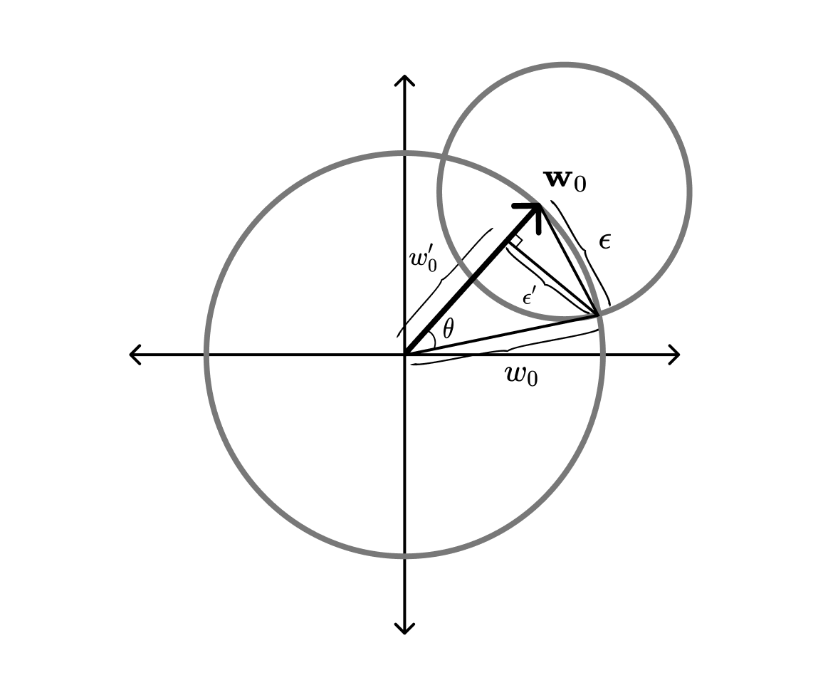
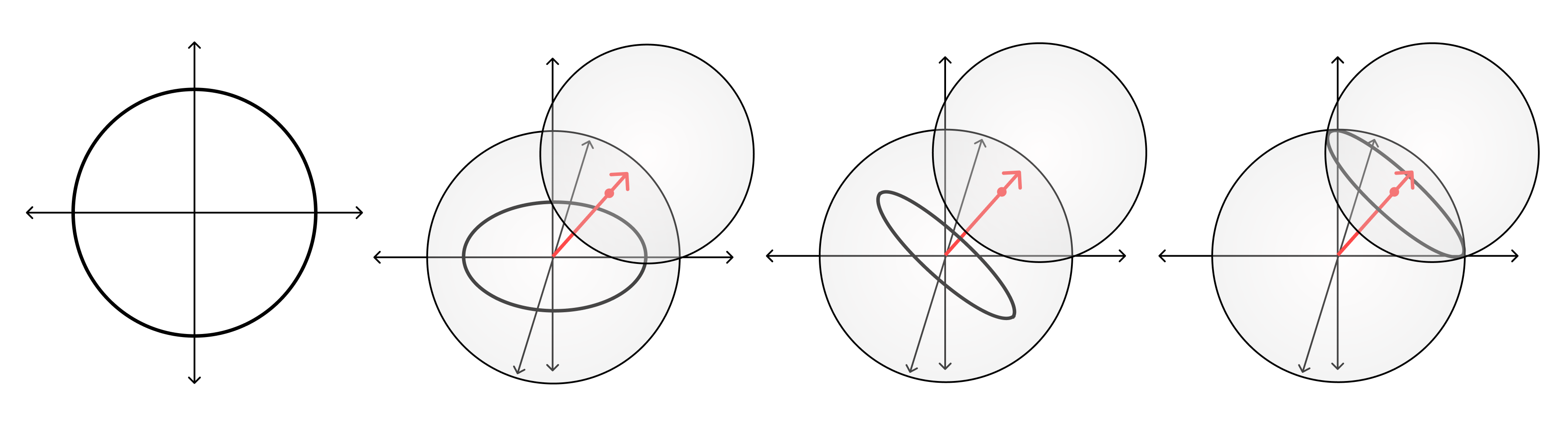
Geometrically, the intersection of a hypersphere $S^D$ of radius $w_0=|\mathbf w_0|$ with a hypersphere $S^D$ of radius $\epsilon$ that is centered at some point on the boundary of the first hypersphere, is a lower-dimensional hypersphere $S^{D-1}$ of a modified radius $\epsilon'$. If we sample uniformly from this lower-dimensional hypersphere, then the resulting points will follow the same distribution over the original hypersphere.

This suggests a procedure to sample from the intersection of the weight initialization hypersphere and the perturbation hypersphere.

First, we sample from a hypersphere of dimension $D-1$ and radius $\epsilon'$ (using the same technique we used to sample the baseline weights). From a bit of trigonometry, see figure below, we know that the radius of this hypersphere will be $\epsilon' = w_0\cos \theta$, where $\theta = \cos^{-1}\left(1-\frac{\epsilon^2}{2w_0^2}\right)$.

Next, we rotate the vector so it is orthogonal to the baseline vector $\mathbf w_0$. This is done with a Householder reflection, $H$, that maps the current normal vector $\hat{\mathbf n} = (0, \dots, 0, 1)$ onto $\mathbf w_0$:

where

and $\hat{\mathbf w}_0 = \frac{\mathbf w_0}{|w_0|}$ is the unit vector in the direction of the baseline weights.

Implementation note: For the sake of tractability, we directly apply the reflection via:

Finally, we translate the rotated intersection sphere along the baseline vector, so that its boundary goes through the intersection of the two hyperspheres. From the figure above, we find that the translation has the magnitude $w_0' = w_0 \cos \theta$.

By the uniform sampling of the intersection sphere and the uniform sampling of the baseline vector, we know that the resulting perturbed vector will have the same distribution as the baseline vector, when restricted to the intersection sphere.

Dynamical Systems

Formally, a dynamical system is a tuple $(\mathcal T, \mathcal M, \Phi)$, where $\mathcal T$ is the "time domain" (some monoid), $\mathcal M$ is the phase space over which the evolution takes place (some manifold), and $\Phi$ is the evolution function, a map,

that satisfies, $\forall x \in \mathcal M, \forall t_{1}, t_{2}\in \mathcal T$,

⁴

Informally, we're usually interested in one of two perspectives:

1. Trajectories of individual points in $\mathcal M$, or
2. Evolution of probability densities over $\mathcal M$.

The former is described in terms of differential equations (for continuous systems) or difference equations (for discrete systems), i.e.,

or

The latter is described in terms of a transfer operator:

Both treatments have their advantages: the particle view admits easier empirical analysis (we just simulate a trajectory), while the latter

In terms of the former, path-sensitivity becomes the question of chaos: do nearby

Varying the Depth

For a fair comparison across network depths, we want to keep the total number of parameters $D$ constant as we increase depth.

Given $n_h$ hidden layers with biases that each have width, $w$, an input dimensionality of $n_\mathrm{in}$, and an output dimensionality of $n_\mathrm{out}$, the total number of parameters is

Lyapunov spectrum

The Lyapunov exponent $\lambda$ quantifies the rate of separation of infinitesimally close trajectories:

If the exponent is positive, then nearby trajectories will diverge, and the dynamics are chaotic. If the exponent is negative, then nearby trajectories will converge

For a $D$-dimensional system, there are $D$ Lyapunov exponents. We often focus exclusively on the maximal Lyapunov exponent because it dominates the overall rate of separation between two neighboring trajectories. However, the full spectrum contains valuable additional information like the rate of entropy production, the fractal dimension, the Hausdorff dimension, and the Lyapunov dimension.

The first major limitation is that the full Lyapunov spectrum is intractable for large $D$. The other major limitation is that the Lyapunov spectrum requires a suitable norm. We can use the l2 norm in $\mathcal W$, but as we already saws what we really care about is measuring distance in $\mathcal F$ with some metric $d : \mathcal F \times \mathcal F \to \mathbb R$.

One option would be to repurpose the loss function $\ell$:

Here, we treat $f_2(x_i)$ as the truth, and use the empirical risk as our distance metric. We could define an analogous distance over either the train or test set. As long as $\ell$ is a suitable metric (or easily converted into a metric through, e.g., symmetrization), $d$ will be too.

This suffers a major downside that two functions will be seen as identical as long as they have the same performance on the dataset in question. They can have totally different performance on unseen examples. Devising suitable distance metrics for neural networks requires more work.

Autocorrelations

The autocorrelation of a random process $\{X_t\}$ is the correlation between two values of that process at different times,

For stationary processes (where $\langle X_t\rangle$ is independent of $t$), this becomes a function of one variable, $\tau=t_2-t_1$,

In the case of training, the dynamics aren't stationary: learning rate schedules and the the "descent" of gradient descent ensures that these correlations will depend on our choice of starting time. However, we're not typically interested in correlations between later time steps. We care about autocorrelations relative to the starting point $t_1=0$.

In practice, the probabilistic and point-wise views are intimately connected: the relevant autocorrelation timescales can often be directly related to the maximal Lyapunov component. These two formulas are only a small sample of the available tooling.

$\mathcal F$ is the space of $p$-integrable functions, $f_w \in \mathcal F$ iff

which is equipped with a metric,

So we exchange evolution over a finite-dimensional $\mathcal W$ with an infinite-dimensional

Footnotes

1. For regression, $\mathcal Y = \mathbb R^N$, for classification, $\mathcal Y \subset \mathbb N$, for self-supervised tasks, we're often interested in $\mathcal Y = \mathcal X$, etc. ↩ ↩²

2. To start, we'll ignore the model hyperparameters. You can view this as either absorbing the hyperparameters into the weights, into the optimizer, or into our choice of $f$. Later, it'll be useful to separate out hyperparameters (i.e., $f: \mathcal X \times \mathcal Y \times \mathcal H \to \mathcal Y$). ↩

3. A quick note on notation: Often, you'll see the dataset denoted with a capital $D$. Here, we're using a lowercase because it'll be useful to treat $\mathbf d$ as an instance of a random variable $\mathbf D$. Similarly for $x$, $y$, and $w$ ($X$, $Y$, and $W$). Even though $x$, $y$, and $w$ are (typically) all vectors, we'll reserve boldface for sets. TODO: Maybe just bite the bullet and bold all of them. ↩

4. It's possible to generalize this further so that $\Phi : U \subseteq (\mathcal T \times \mathcal M) \to \mathcal M$, but this won't be necessary for us. ↩