Towards Developmental Interpretability
This is an link post, originally posted at https://www.lesswrong.com/posts/TjaeCWvLZtEDAS5Ex/towards-developmental-interpretability.
This is an link post, originally posted at https://www.lesswrong.com/posts/TjaeCWvLZtEDAS5Ex/towards-developmental-interpretability.
This is an link post, originally posted at https://www.lesswrong.com/posts/gq9GR6duzcuxyxZtD/approximation-is-expensive-but-the-lunch-is-cheap.
In the world of finance, quants develop trading algorithms to gain an edge in the market. As these algorithms are deployed and begin to interact with each other, they change market dynamics and can end up in different environments from what they were developed for. This leads to continually degrading performance and the ongoing need to develop and refine new trading algorithms. When deployed without guardrails, these dynamics can lead to catastrophic failures such as the flash crash of 2010, in which the stock market temporarily lost more than one trillion dollars.
This is an extreme example of distribution shift, where the data a model is deployed on diverges from the data it was developed on. It is key concern within the field of AI safety, where a concern is that mass-deployed SOTA models could lead to similar catastrophic outcomes with impacts not limited to financial markets.
In the more prosaic setting, distribution shift is concerned with questions like: Will a self-driving car trained in sunny daytime environments perform well when deployed in wet or nighttime conditions? Will a model trained to diagnose X-rays transfer to a new machine? Will a sentiment analysis model trained on data from one website work when deployed on a new platform?
In this document, we will explore this concept of distribution shift, discuss its various forms and causes, and explore some strategies for mitigating its effects. We will also define key related terms such as out-of-distribution data, train-test mismatch, robustness, and generalization.
To understand distribution shift, we must first understand the learning problem.
The dataset. In the classification or regression setting, there is a space of inputs, , and a space of outputs, , and we would like to learn a function ("hypothesis") . We are given a dataset, , of samples of input-output behavior and assume that each sample is sampled independently and identically from some "true" underlying distribution, .
The model. The aim of learning is to find some optimal model, , parametrized by , where optimal is defined via a loss function that evaluates how different a prediction is from the true outcome .
Empirical risk minimization. We would like to find the model that minimizes the expected loss over all possible input-output pairs; that is, the population risk:
However, we do not typically have direct access to (and even with knowledge of the integral would almost certainly be intractable). Instead, as a proxy for the population risk, we minimize the loss averaged over the dataset, which is known as the empirical risk:
Training and testing. In practice, to avoid overfitting we split the dataset into a training set, , and a test set, . We train the model on but report performance on . If we want to find the optimal hyperparameters in addition to the optimal parameters, we may further split part of the dataset into additional cross-validation sets. Then, we train on the training set, select hyperparameters via the cross-validation sets, and report performance on a held-out test set.
Deployment. Deployment, rather than testing, is the end goal. At a first pass, distribution shift is simply when the performance on the training set or test set is no longer predictive of performance during deployment. Most of the difficulty in detecting and mitigating this phenomenon comes down to their being few or no ground-truth labels, , during deployment.
Distribution shift. Usually, distribution shift refers to when the data in the deployment environment is generated by some distribution, that differs from the distribution, , responsible for generating the dataset. Additionally, it may refer to train-test mismatch in which the distribution generating the training set, , differs from the distribution generating the test set, .
Train-test mismatch. Train-test mismatch is easier to spot than distribution shift between training and deployment, as in the latter case there may be no ground truth to compare against. In fact, train-test mismatch is often intentional. For example, to deploy a model on future time-series data, one may split the training and test set around a specific date. If the model translates from historical data in the training set to later data in the test set, it may also extend further into the future.
Generalization and robustness. Understanding how well models translate to unseen examples from the same distribution (generalization or concentration) is different to understanding how well models translate to examples from a different distribution (robustness). That's because distribution shift is not about unbiased sampling error; given finite sample sizes, individual samples will necessarily differ between training, test, and deployment environments. (If this were not the case, there would little point to learning.) Authors may sometimes muddy the distinction (e.g., "out-of-distribution generalization"), which is why we find it worth emphasizing their difference.
Out-of-distribution. "Distribution shift" is about bulk statistical differences between distributions. "Out-of-distribution" is about individual differences between specific samples. Often, an "out-of-distribution sample" refers to the more extreme case in which that sample comes from outside the training or testing domain (in which case, "out-of-domain" may be more appropriate). See, for example, the figure below.
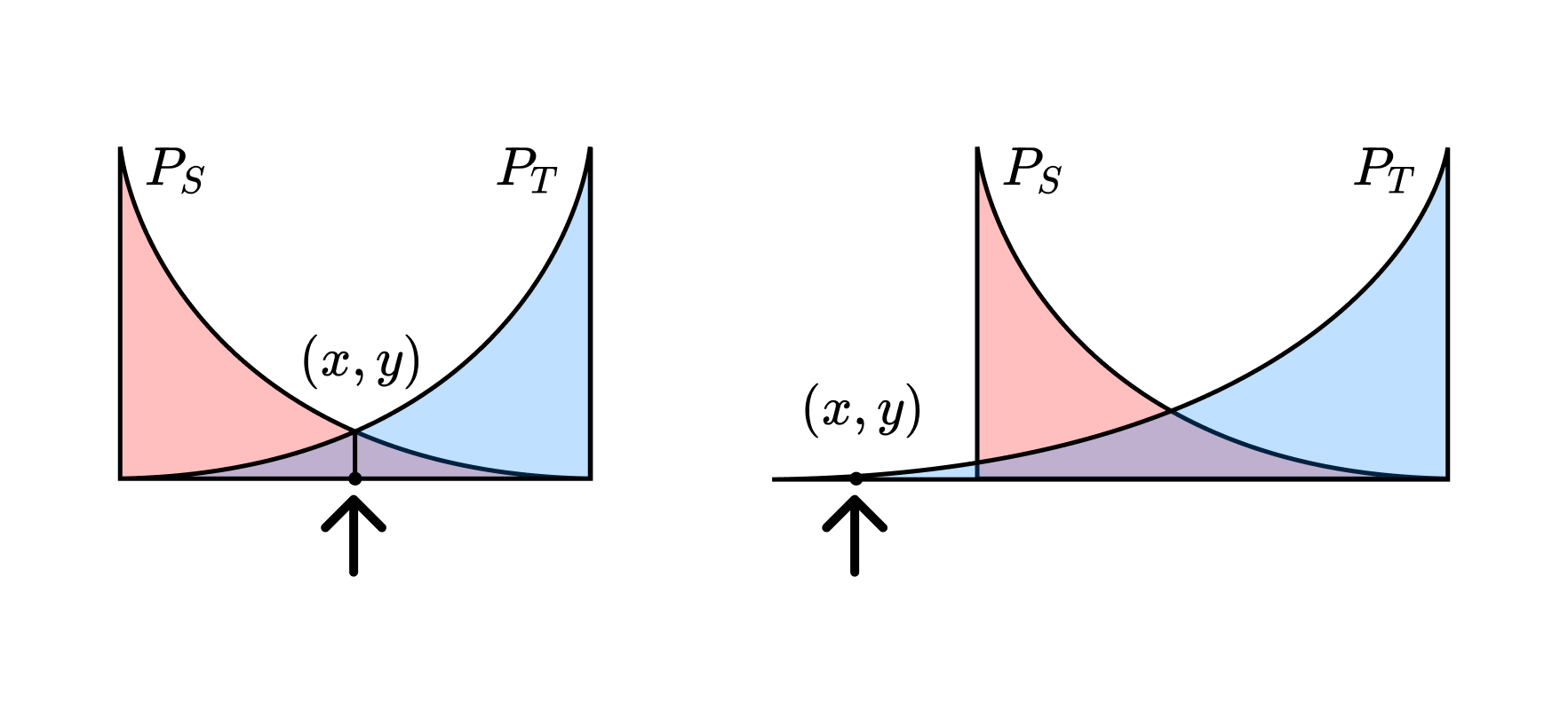
The main difference between "distribution shift" and "out-of-distribution" is whether one is talking about bulk properties or individual properties, respectively. On the left-hand side, the distributions differ, but the sample is equally likely for either distribution. On the right-hand side, the distributions differ, and the sample is out-of-domain.
Non-stationarity. Distribution shift can result from the data involving a temporal component and the distribution being non-stationary, such as when one tries to predict future commodity prices based on historical data. Similar effects can occur as a result of non-temporal changes (such as training a model on one geographical area or on a certain source of images before applying it elsewhere).
Interaction effects. A special kind of non-stationarity, of particular concern within AI safety, is the effect that the model has in deployment on the systems it is interacting with. In small-scale deployments, this effect is often negligible, but when deployed on massive scales, this effect (as in finance where automated bots can move billions of dollars) the consequences can become substantial.
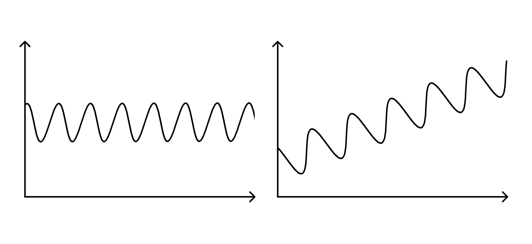
Stationary vs. non-stationary data.
Sampling bias. Though distribution shift does not refer to unbiased sampling error, it can refer to the consequences of biased sampling error. If one trains a model on the results of an opt-in poll, it may not perform well when deployed to the wider public. These kinds of biases are beyond the reach of conventional generalization theory and up to the study of robustness.
The true data-generating distribution can be factored,
which helps to distinguish several different kinds of distribution shift.
Covariate shift is when is held constant while changes. The actual transformation from inputs to outputs remains the same, but the relative likelihoods of different inputs changes. This can result from any of the causes listed above.
Label shift is the reverse of covariate shift, where is held constant while changes. Through Bayes' rule and marginalization, covariate shift induces a change in and vice-versa, so the two are related, but not exactly the same: assuming that either remains constant or that remains constant are not the same assumptions.
Concept drift is where is held constant while changes. The distribution over inputs is unchanged while the transformation from inputs to outputs changes. In practice, it is rarely the case that a distribution shift falls cleanly into one of these three categories. Still, this taxonomy can be useful as a practical approximation.
Internal covariate shift is a phenomenon specific to deep neural networks, where sampling error between batches can induce large changes in the distribution of internal activations, especially for those activations deeper in the model. That said, this is not a distribution shift in the classical sense, which refers to a change ).
Techniques for mitigating distribution shift include data augmentation, adversarial training, regularization techniques like dropout, domain adaptation, model calibration, mechanistic anomaly detection, batch normalization for internal covariate shift, online learning, and even simple interventions like using larger, pre-trained models.
In this document, we discussed the importance of distribution shift in machine learning, its causes, and strategies for mitigating its effects. We also defined key terms such as distribution shift, out-of-distribution, and train-test mismatch. Addressing distribution shift
This is an link post, originally posted at https://www.lesswrong.com/posts/HtxLbGvD7htCybLmZ/singularities-against-the-singularity-announcing-workshop-on.
This is an link post, originally posted at https://www.lesswrong.com/posts/zuYRyC3zghzgXLpEW/empirical-risk-minimization-is-fundamentally-confused.