How to Perturb Weights

I'm running a series of experiments that involve some variation of: (1) perturb a weight initialization; (2) train the perturbed and baseline models in parallel, and (3) track how the perturbation grows/shrinks over time.

Naively, if we're interested in a perturbation analysis of the choice of weight initialization, we prepare some baseline initialization, $\mathbf w_0$, and then apply i.i.d. Gaussian noise, $\boldsymbol \delta$, to each of its elements, $\delta_i \sim \mathcal N(0, \epsilon^2)$. (If we want, we can let this vary layer-by-layer and let it depend on, for example, the norm of the layer it's being applied to.)

The problem with this strategy is that the perturbed weights $\mathbf w = \mathbf w_0 + \boldsymbol\delta$ are, in general, no longer sampled from the same distribution as the baseline weights.

There is nothing wrong with this per se, but it introduces a possible confounder (the thickness). This is especially relevant if we're interested specifically in the question of how behavior changes with the size of a perturbation, this problem introduces a possible confounder. As responsible experimentalists, we don't like confounders.

Fortunately, there's an easy way to "clean up" Kaiming He to make it better suited to this perturbative analysis.

Kaiming initialization lives in a hyperspherical shell

Consider a matrix, $\mathbf w^{(l)}$, representing the weights of a particular layer $l$ with shape $(D_\mathrm{in}^{(l)}, D_\mathrm{out}^{(l+1)})$. $D_\mathrm{in}^{(l)}$ is also called the fan-in of the layer, and $D_\mathrm{in}^{(l+1)}$ the fan-out. For ease of presentation, we'll ignore the bias, though the following reasoning applies equally well to the bias.

We're interested in the vectorized form of this matrix, $\vec w^{(l)} \in \mathbb R^{D^{(l)}}$, where $D^{(l)} =D_\mathrm{in}^{(l)} \times D_\mathrm{out}^{(l+1)}$.

In Kaiming initialization, we sample the components, $w_i^{(l)}$, of this vector, i.i.d. from a normal distribution with mean 0 and variance $\sigma^2$ (where $\sigma^2 = \frac{2}{D_\mathrm{in}^{(l)}}$).

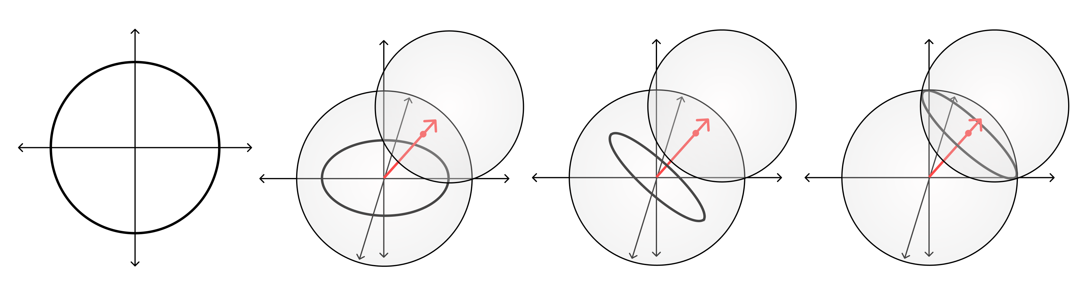
Geometrically, this is equivalent to sampling from a hyperspherical shell, $S^{D-1}$ with radius $\sqrt{D}\sigma$ and (fuzzy) thickness, $\delta$. (Ok, so technically, because the radius can vary from layer-to-layer, it's a hyperellipsoidal shell.)

This follows from some straightforward algebra (dropping the superscript $l$ for simplicity):

and

So the thickness as a fraction of the radius is

where the last equality follows from the choice of $\sigma$ for Kaiming initialization.

This means that for suitably wide networks ($D_\mathrm{in}^{(l)} \to \infty$), the thickness of this shell goes to $0$.

Taking the thickness to 0

This suggests an alternative initialization strategy. What if we immediately take the limit $D_\text{in}^{(l)} \to \infty$, and sample directly from the boundary of a hypersphere with radius $\sqrt{D}\sigma$, i.e., modify the shell thickness to be $0$.

This can easily be done by sampling each component from a normal distribution with mean 0 and variance $1$ and then normalizing the resulting vector to have length $\sqrt{D}\sigma$ (this is known as the Muller method).

Perturbing Weight initialization

The modification we made to Kaiming initialization was to sample directly from the boundary of a hypersphere, rather than from a hyperspherical shell. This is a more natural choice when conducting a perturbation analysis, because it makes it easier to ensure that the perturbed weights are sampled from the same distribution as the baseline weights.

Geometrically, the intersection of a hypersphere $S^D$ of radius $w_0=|\mathbf w_0|$ with a hypersphere $S^D$ of radius $\epsilon$ that is centered at some point on the boundary of the first hypersphere, is a lower-dimensional hypersphere $S^{D-1}$ of a modified radius $\epsilon'$. If we sample uniformly from this lower-dimensional hypersphere, then the resulting points will follow the same distribution over the original hypersphere.

This suggests a procedure to sample from the intersection of the weight initialization hypersphere and the perturbation hypersphere.

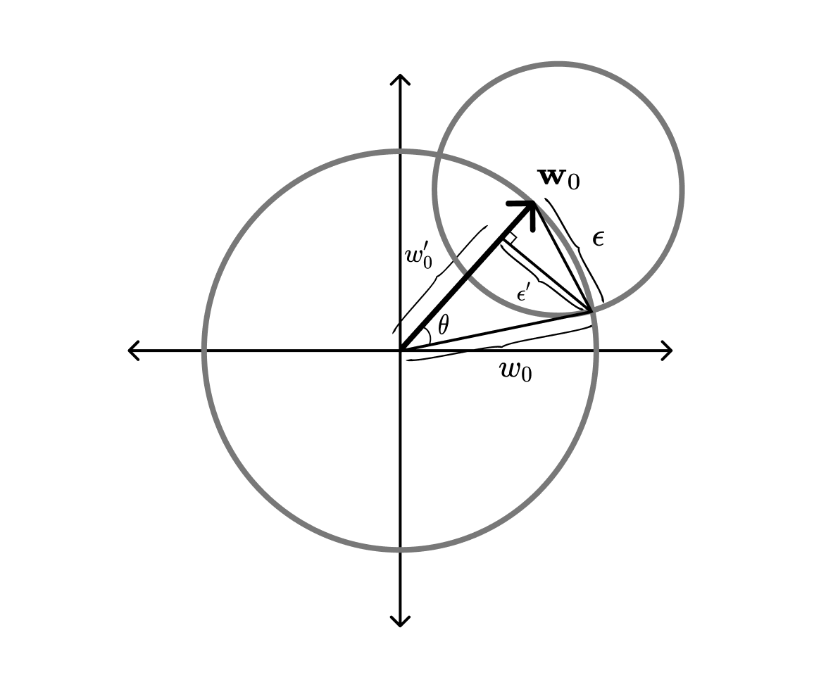
First, we sample from a hypersphere of dimension $D-1$ and radius $\epsilon'$ (using the same technique we used to sample the baseline weights). From a bit of trigonometry, see figure below, we know that the radius of this hypersphere will be $\epsilon' = w_0\cos \theta$, where $\theta = \cos^{-1}\left(1-\frac{\epsilon^2}{2w_0^2}\right)$.

Next, we rotate the vector so it is orthogonal to the baseline vector $\mathbf w_0$. This is done with a Householder reflection, $H$, that maps the current normal vector $\hat{\mathbf n} = (0, \dots, 0, 1)$ onto $\mathbf w_0$:

where

and $\hat{\mathbf w}_0 = \frac{\mathbf w_0}{|w_0|}$ is the unit vector in the direction of the baseline weights.

Implementation note: For the sake of tractability, we directly apply the reflection via:

Finally, we translate the rotated intersection sphere along the baseline vector, so that its boundary goes through the intersection of the two hyperspheres. From the figure above, we find that the translation has the magnitude $w_0' = w_0 \cos \theta$.

By the uniform sampling of the intersection sphere and the uniform sampling of the baseline vector, we know that the resulting perturbed vector will have the same distribution as the baseline vector, when restricted to the intersection sphere.