Random Walks on Hyperspheres

Neural networks begin their lives on a hypersphere.

As it turns out, they live out the remainder of their lives on hyperspheres as well. Take the norm of the vectorized weights, $\mathbf w$, and plot it as a function of the number of training steps. Across many different choices of weight initialization, this norm will grow (or shrink, depending on weight decay) remarkably consistently.

In the following figure, I've plotted this behavior for 10 independent initializations across 70 epochs of training a simple MNIST classifier. The same results hold more generally for a wide range of hyperparameters and architectures.

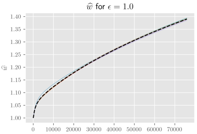
The norm during training, divided by the norm upon weight initialization. The parameter ϵ controls how far apart (as a fraction of the initial weight norm) the different weight initializations are.

All this was making me think that I disregarded Brownian motion as a model of SGD dynamics a little too quickly. Yes, on lattices/planes, increasing the number of dimensions makes no difference to the overall behavior (beyond decreasing the variance in how displacement grows with time). But maybe that was just the wrong model. Maybe Brownian motion on hyperspheres is considerably different and is actually the thing I should have been looking at.

Asymptotics ($t, n \to \infty$)

We'd like to calculate the expected displacement (=distance from our starting point) as a function of time. We're interested in both distance on the sphere and distance in the embedding space.

Before we tackle this in full, let's try to understand Brownian motion on hyperspheres in a few simplifying limits.

Unlike the Euclidean case, where having more than one dimension means you'll never return to the origin, living on a finite sphere means we'll visit every point infinitely many times. The stationary distribution is the uniform distribution over the sphere, which we'll denote $\mathcal U^{(n)}$ for $S^n$.

So our expectations end up being relatively simple integrals over the sphere.

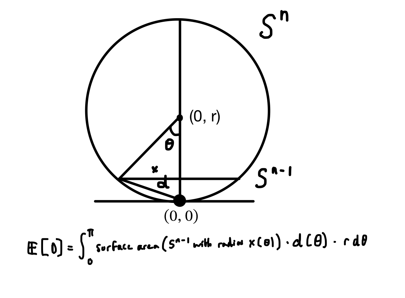
The distance from the pole at the bottom to any other point on the surface depends only on the angle from the line intersecting the origin and the pole to the line intersecting the origin and the other point,

This symmetry means we only have to consider a single integral from the bottom to to the top of $S^{n-1}$ "slices." Each slice has as much probability associated to it as the corresponding $S^{n-1}$ has surface area times the measure associated to $\theta$ ($=r\ \mathrm d \theta$). This surface area varies with the angle from the center, as does the distance of that point from the origin. Put it together and you get some nasty integrals.

From this point on, I believe I made a mistake somewhere (the analysis for $n \to \infty$ is correct).

If we let $S_{n}(x)$ denote the surface area of $S^{n}$ with radius $r$, we can fill in the formula from Wikipedia:

Filling in $x(\theta) =r \sin\theta$, we get an expression for the surface area of each slice as a function of $\theta$,

so the measure associated to each slice is

$n \to \infty$

We can simplify further, as $n\to\infty$, the $\sin^{n-1}(\theta)$ will tend towards a "comb function," that is zero everywhere except for $\theta = (m + 1/2)\pi$ for integer $m$, where it is equal to $1$ if $m$ is even, and $-1$ if $m$ is odd.

Within the above integration limits $(0, \pi)$, this means all of the probability becomes concentrated at the middle, where $\theta=\pi/2$.

So in the infinite-dimensional limit, the expected distance from the origin is the distance between a point on the middle and one of its poles, which is $\sqrt{2} r$.

General case

An important lesson I've learned here is: "try more keyword variations in Google Scholar and Elicit before going off and solving these nasty integrals yourself because you will probably make a mistake somewhere and someone else has probably already done the thing you're trying to do."

Anyway, here's the thing where someone else has already done the thing I was trying to do. [1] gives us the following form for the expected cosine of the angular displacement with time:

$\langle\cos \theta(t)\rangle=\exp \left(-D(n-1) t / R^2\right).$

A little trig tells us that the expected displacement in the embedding space is

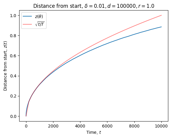
which gives us a set of nice curves depending on the diffusion constant $D$:

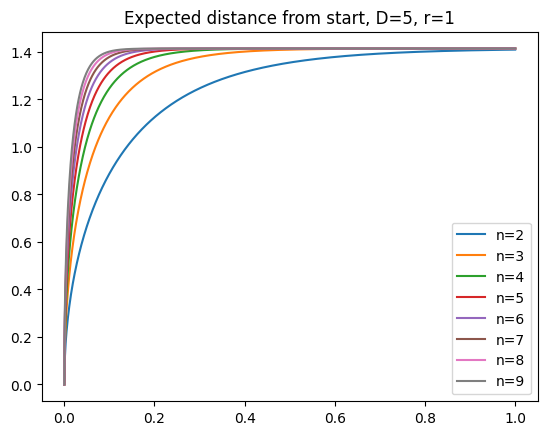
The major difference with Brownian motion on the plane is that expected displacement asymptotes at the limit we argued for above ($\sqrt{2} r$).

When I had initially looked at curves like the following (this ones from [numerical simulation](https://github.com/jqhoogland/experiminis/blob/main/brownian_hyperspheres.ipynb, not the formula), I thought I had struck gold.

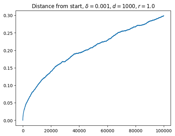
I've been looking for a model that predicts square root like growth at the very start, followed by a long period of nearly linear growth, followed by asymptotic behavior. Eyeballing this, it looked like my searching for the long plateau of linear growth had come to an end.

Of course, this was entirely wishful thinking. Human eyes aren't great discriminators of lines. That "straight line" is actually pretty much parabolic. As I should have known (from the Euclidean nature of manifolds), the initial behavior is incredibly well modeled by a square root.

As you get further away from the nearly flat regime, the concavity only increases. This is not the curve I was looking for.

So my search continues.