Review of Generalization

NOTE: Work in Progress

Outline

• Warm-up: MSE & bias-variance trade-offs.
• Generalization = Simplicity.
  • Solomonoff induction,
  • Complexity measures
    • BIC/MDL, AIC
    • VC dimension & structural risk minimization
    • Rademacher complexity
• Early Stopping
  • NTK
• Problems:
  • Vacuous bounds (Zhang et al. 2017). Always zero training error. Any optimizer (even stupid ones). Crazily convex loss spots. Even with regularization
• From functions to probabilities
  • Gibbs measure
  • PAC-Bayes bounds
    • NNs Dziugaite & Roy 2017
  • Singular learning theory, WAIC
• Mingard-style “Bayesian inference”

Misc:

• SGD & Basin broadness
• Heavy-tailed random matrix theory (implicit self-regularization)
• Double descent & grokking
• Recent Anthropic work It’s non-obvious that (l2) regularization chooses simpler functions in NNs. (Polynomial regression is one thing).

"Regular" learning theory (RLT) predicts that overparametrized deep neural networks (DNNs) should overfit. In practice, the opposite happens: deeper networks perform better and generalize further. What's going on?

The consensus is still out, but different strands of research appear to be converging on a common answer: DNNs don't overfit because they're not actually overparametrized; SGD and NN's symmetries favor "simpler" models whose effective parameter counts are much lower than the externally observed parameter count. Generality comes from a kind of internal model selection where neural networks throw out unnecessary expressivity.

In this post, I'll make that statement more precise. We'll start by reviewing what RLT has to say about generalization and why it fails to explain generalization in DNNs. We'll close with a survey of more recent attempts at the learning theory of DNNs with particular emphasis on "singular" learning theory (SLT).

Intro to Statistical Learning Theory

Before we proceed, we need to establish a few definitions. Statistical learning theory is often sloppy with its notation and assumptions, so we have to start at the basics.

In this post, we'll focus on a (self-)supervised learning task. Given an input $x \in \mathcal X$, we'd like to predict the corresponding output $y \in \mathcal Y$. This relationship is determined by an unknown "true" pdf $q(z) = q(x, y)$ over the joint sample space $\mathcal Z = \mathcal X \times \mathcal Y$.

If we're feeling ambitious, we might directly approximate the true joint distribution with a generative model $p(x, y|w)$ that is parametrized by weights $w \in \mathcal W \subseteq \mathbb R^D$. If it's tractable, we can marginalize this joint distribution to obtain the marginal and conditional distributions. ¹

If we're feeling less ambitious, we might go ahead with a discriminative model of the conditional distribution, $p(y| x, w)$. (In the case of regression and classification, we're interested in inferring target values and labels from future samples, so we may not care all that much about $q(x)$ and $q(x|y)$.)

And if we're feeling unambitious (as most machine learning theorists are), it may be enough to do direct inference with a discriminant function — i.e., to find a deterministic function that maps inputs to outputs, $f_w: \mathcal X \to \mathcal Y$.²

In the case of regression, this is justified on the (only occasionally reasonable) assumption that the error is i.i.d. sampled from a Gaussian distribution. In other words, the discriminative model is defined in terms of $f$ as:

Machine learning usually begins with discriminant functions. Not only is this often easier to implement, but it offers some additional flexibility in the kinds of functions we can model because we optimize arbitrary loss functions that are unmoored from Bayesian-grounded likelihoods or posteriors.³

This flexibility comes at a cost: without the theoretical backing, it's more difficult to reason systematically about what's actually going on. The loss functions and regularizers of machine learning often end up feeling ad hoc and unsupported because they are. Or at least they will be until section 3.

As a result, we'll find it most useful to work at the intermediate level of analysis, in terms of discriminant models.

What Is Learning, Anyway?

The strength of the Bayesian framing is that for some prior over weights, $\phi(w)$, and a dataset $\mathbf d^{(n)} \in \mathcal Z^n$ of samples $\{(x_i, y_i)\}_{i=1}^n$, we can "reverse" the likelihood (assuming each sample is sampled i.i.d. from $p(x, y)$),

to obtain the a posteriori distribution,

where $Z_n$ is the evidence (or partition function),

The aim of "learning" is to make our model $p(y|x, w)$ as "close" as possible to the truth $q(y|x)$.

In the probabilistic formulation, the natural choice of "distance" is the Kullback-Leibler divergence (which is not actually a distance):

where the second equality follows from defining $q(x, y|w) = q(y|x, w) \cdot p(x)$.

Formally, the aim of learning is to solve the following:

We say $p(y|x)$ is realizable iff $K(w^*) = 0$, in which case we call $w^*$ the "true" parameters.

At this point, we run into a bit of a problem: we can't actually compute the expectations $\langle \cdot\rangle_{X, Y}$ since we don't know $p(x, y)$ (and even if we did, the integration would likely be intractable). Instead, we have to resort to empirical averages over a dataset,. ³

Maximum Likelihood Estimation is KL-Divergence Minimization

Example: Regression & Mean-Squared Error

Fortunately, there's a more general and principled way to recover discriminant models from discriminant functions than the assumption of isotropic noise, as long as we're willing to relax Bayes' rule.

First, we introduces a parameter $\beta \geq 0$ that controls the tradeoff between prior and likelihood to obtain the tempered Bayes update [1],⁴

$p_\beta(w|\mathbf d) \propto p(\mathbf d| w)^{\beta}p(w),$

where $\mathbf d$ is a dataset of samples $\{(x_{i},y_{i})\}_{i=1}^n$, and the likelihood is obtained by assuming each sample is distributed i.i.d. according to $p(x_{i}, y_{i}|w)$ s.t. $p(\mathbf d|w) = \prod_{i=1}^{n}p(x_{i}, y_{i}|w)$.

Next, we replace the tempered likelihood with a general loss function

The real-world is noisy, and pure function approximation can't account for this.

To remedy this, it's common to model any departure from our deterministic predictions, $\hat y = f_w(x)$, as isotropic noise, e.g., $q(y|x, w) = \mathcal N(y| f_w(x), \sigma^2)$.

Physically, we may expect the underlying process to be deterministic (given by a "true" function $f^*$) with noise creeping in through some unbiased measurement error $\epsilon \sim \mathcal N(0, \sigma^2)$.

For Gaussian noise, the NLL works out to:

Assuming isotropic Gaussian noise in a regression setting, we see that MLE simplifies to minimizing the mean squared error (up to some overall constant and scaling).

To make MLE more Bayesian, you just multiply the likelihood by some prior over the weights, to obtain maximum a posteriori estimation (MAP): $p(w|\mathbf d) \propto p(\mathbf d|w)\phi(w).$ If we enforce a gaussian prior with precision $\alpha$, the loss gains a regularization term (weight decay), $\frac{\alpha}{2}w^T w$ to the loss function. [2]

Gibbs Generalization Error

Todo

What Is Generalization, Anyway?

Consider the empirical probability distribution,

where $\delta(\cdot)$ is a delta function appropriate to the sample space.

Although this will converge to the true distribution as $N\to\infty$, for any finite $N$, we encounter sampling error. This problem is particularly pronounced for unseen samples: $q_D(z)$ may (and almost always does) assign zero probability to samples that have non-zero probability under the true distribution.

The fundamental challenge of generalization is to make predictions about these unseen samples. Let's make this more precise.

Given some loss function $\ell: Y \times Y \to \mathbb R$, we're interested in how $\ell$ performs on future samples, as measured by the expected risk or generalization error,

However, we can only estimate this performance on on the available dataset via the empirical risk,

where $\overline \cdot$ denotes an empirical average over the dataset, $\mathbf d$.

Our problem is that the true generalization error is unknowable. So, in practice, we split our dataset into a training set, $\mathbf s$, and test set, $\mathbf e$, respectively. We learn our parameters $w$ via the training set, and then estimate the generalization error on the test set. That's where we encounter our first major confusion.³

You see, besides the generalization error, there's the distinct notion of the generalization gap,

Whereas generalization error is about absolute performance on the true distribution, the generalization gap is about relative performance between the training and test sets. Generalization error combines both "performance" and "transferability" into one number, while the generalization gap is more independent of "performance" — past a certain threshold, any amount of test-set performance is compatible with both a low and high generalization gap.

For the remainder of this post, I'll focus on the generalization gap. It's not absolute performance we're interested in: universal approximation theorems tell us that we should expect excellent training performance for neural networks. The less obvious claim is why this performance should transfer so well to novel samples.

---

Yes, more data means better generalization, but that's not what we're talking about.

In the limit $N\to \infty$, the empirical risk converges to expected risk, and both generalization error and gap will fade away: $\epsilon_g \to 0,\quad \epsilon_g^2 \to 0 \quad \text{as} \quad N \to \infty.$ So obviously the larger datasets that have accompanied the deep learning boom explain some of the improvement in generalization.

PAC Learning

Established by Valiant (1984) [3], Probably Approximately Correct (PAC) learning establishes upper bounds for the risk $I[f]$. In its simplest form, it states that, for any choice of $\epsilon$ ("probably") a predictor, $f$, will have its risk bounded by some $\delta$ ("approximately correct"):

Originally, PAC learning included the additional assumption that the predictor was polynomial in $N$ and $1/\epsilon$, but this has been relaxed to refer to any bound holding with high probability.

Still, it's not a full explanation as typical networks can easily memorize the entire training set (even under random labelings [4]).

---

MSE & Bias-variance tradeoff

In the case of isotropic noise (where our loss function is the MSE), the generalization error of a model is:

In other words, it is the (l2) distance between our predictions and the truth averaged over the true variables $X \times Y$. The bias-variance decomposition splits the generalization error into a bias term,

which measures the average difference between predictions and true values, a variance term,

which measures the spread of a model's predictions for a given point in the input space, and an irreducible error due to the inherent noise in the data. (For Gaussian noise, the irreducible error is $\sigma^2$.)

In order to achieve good generalization performance, a model must have low bias and low variance. This means that the model must be complex enough to capture the underlying patterns in the data, but not so complex that it overfits the data and becomes sensitive to noise. In practice, these two forces are at odds, hence "tradeoff."

---

Generalization is about simplicity

A common assumption across the entire statistical learning theory literature is that of simple functions generalizing better. It's worth spending a second to understand why we should expect this assumption to hold.

Occam's Razor

"Entities must not be multiplied beyond necessity".

Occam's razor is the principle of using the simplest explanation that fits the available data. If you're reading this, you probably already take it for granted.

Solomonoff Induction

Algorithmic complexity theory lets us define a probability distribution over computable numbers,

$p(x)= \sum_{p}2^{-K(p)},$ where $K(\cdot)$ is the (prefix) Kolmogorov complexity. The probability of any given number is the probability that a uniform random input tape on some Universal Turing Machine outputs that number. Unfortunately, the halting problem makes this just a tad uncomputable. Still, in principle, this allows a hypercomputer to reason from the ground up what the next entry in a given sequence of numbers should be.

Bayesian/Akaike Information Criterion

One of the main strengths of the Bayesian frame is that it lets enforce a prior $\varphi(w)$ over the weights, which you can integrate out to derive a parameter-free model:

One of the main weaknesses is that this integral is often almost always intractable. So Bayesians make a concession to the frequentists with a much more tractable Laplace approximation (i.e., you approximate your model as quadratic/gaussian in the vicinity of the maximum likelihood estimator (MLE), $w^{(0)}$):

where $I(w)$ is the Fisher information matrix:

From this approximation, a bit more math gives us the Bayesian information criterion (BIC):

The BIC (like the related Akaike information criterion) is a criterion for model selection that penalizes complexity. Given two models, the one with the lower BIC tends to overfit less (/"generalize better").

That is, simpler models (with fewer parameters) are more likely in approximate Bayesian inference. We'll see in the section on singular learning theory that the BIC is unsuitable for deep neural networks, but a generalized version, the Widely Applicable Bayesian Information Criterion (WBIC) will pick up the slack.

Minimum Description Length

The BIC is formally equivalent to MDL. TODO

Maximum Entropy Modeling

TODO

Classic Learning Theory

As we've seen in the previous section, the question of how to generalize reduces to the question of how to find simple models that match the data.

In classical learning theory, the answer to this is easy: use fewer parameters, include a regularization term, and enforce early stopping. Unfortunately, none of these straightforwardly help us out with deep neural networks.

For one, double descent tells us that the relation between parameter count and generalization is non-monotonic: past a certain number of parameters, generalization error will start decreasing. Moreover, a large number of the complexity measures we've seen are extensive (they scale with model size). That suggests they're not suited to the task.

As for regularization, it gets more complicated. That regularization on polynomial regression leads to simpler functions is straightforward. That regularization on deep neural networks leads to simpler models is less obvious. Sure, a sparse l1 regularizer that pushes weights to zero seems like it would select for simpler models. But a non-sparse l2 regularizer? Linking small parameters to simple functions will require more work. A deeper problem is that DNNs can memorize randomly labeled data even with regularizers [5]. Why then, do DNNs behave so differently on correctly labeled (/well-structured) data

Other forms of regularization like dropout are more understandable: they explicitly select for redundancy which collapses the effect parameter count.

Finally, early stopping doesn't seem to work with the observation of grokking: in certain models, training loss and test loss may plateau (at a poor generalization gap) for many epochs before training loss suddenly sharply decreasing (towards a much better generalization gap).

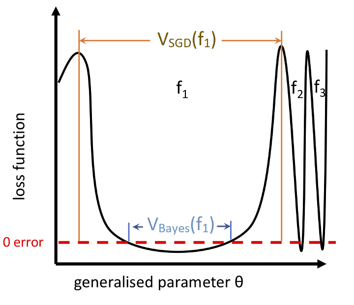
SGD Favors Flat Minima

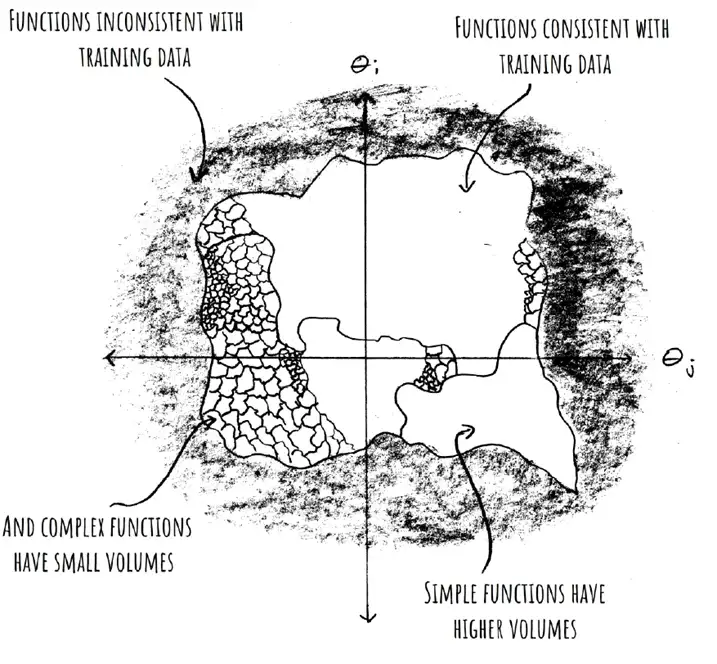
• $P_\beta(f)$ is the probability that $M$ expresses $f$ on $D$ upon a randomly sampled parametrization. This is our "prior"; it's what our network expresses on initialization.
• $V_\beta(f)$ is a volume with Gaussian measure that equals $P_\beta(f)$ under Gaussian sampling of network parameters.
  • This is a bit confusing. We're not talking about a continuous region of parameter space, but a bunch of variously distributed points and lower-dimensional manifolds. Mingard never explicitly points out why we expect a contiguous volume. That or maybe it's not necessary for it to be contiguous
• $\beta$ denotes the "Bayesian prior"
• $P_\text{opt}(f|S)$ is the probability of finding $f$ on $E$ under a stochastic optimizer like SGD trained to 100% accuracy on $S$.
• $P_\beta(f|S) = \frac{P(S|f) P_\beta(f)}{P_\beta(S)},$ is the probability of finding $f$ on $E$ upon randomly sampling parameters from i.i.d. Gaussians to get 100% accuracy on $S$.
  • This is what Mingard et al. call "Bayesian inference"
  • $P(S|f)=1$ if $f$ is consistent with $S$ and $0$ otherwise I.e.: Hessians with small eigenvalues.

Flat minima seem to be linked with generalization:

• Hochreiter and Schmidhuber, 1997a; Keskar et al., 2016; Jastrzebski et al., 2018; Wu et al., 2017; Zhang et al., 2018; Wei and Schwab, 2019; Dinh et al., 2017.

SGD

Problems:

• Suitable reparametrizations can change flatness without changing computation.

Initialization Favors "simple" functions

Mingard 2021

• Levin et al. tell us that many real-world maps satisfy $P(f) \lesssim 2^{-b\tilde K(f)+a}$, where $\hat K$ is a computable approximation of the true Kolmogorov complexity $K(f)$.
• Empirically, maps of the form $f:\{0, 1\}^n \to \{0, 1\}$ satisfy a similar upper bound using a computable complexity measure (CSR).
• This is an upper bound, not more than that!
• The initialization acts as our prior in Bayesian inference.

SGD Performs Hidden Regularization

Mingard 2020

1. **Bayesian inference preserves the "simplicity" of the prior.
2. SGD performs a kind of "Bayesian inference"
   • You can approximate $P_\beta(f)$ with Gaussian Processes.
   • Mingard's main result is that $P_\text{opt}(f|S) \approx P_\beta(f|S)$ appears to hold for many datasets (MNIST, Fashion-MNIST, IMDb movie review, ionosphere), architectures (Fully connected, Convolutional, LSTM),  optimizers (SGD, Adam, etc.), training schemes (including overtraining) and optimizer hyperparameters (e.g. batch size, learning rate).
   • Optimizer hyperparameters matter much less than $P_\beta(f|S)$

Singular Learning theory

Glossary

• $f^*$ is the true function
• $f$ is some implemented function
• $M$ is our neural network
• $D$ is a dataset of pairs $\{(x_i, y_i)\}_{i=1}^N$
• $S, E \subset D$ are the training & test sets, respectively.

Learnability

• PAC in original formulation: simpler functions are easier to learn (polynomial time)

Usually, the true relation is probabilistic. In this case, we're not interested in a deterministic mapping $f^*$ from elements of $\mathcal X$ to elements $\mathcal Y$, but a probability distribution, $q(x, y)$, which relates random variables $X$ and $Y$ (where $\mathcal X$ and $\mathcal Y$ are the associated sample spaces).

We don't have direct access to $q(x, y)$, but we do have access to a dataset of samples, $\mathbf D = \{(X_i, Y_i)\} _ {i=1}^n$, which is itself a random variable. We specify some loss function, $\ell$, $\mathcal Y \times \mathcal Y \to\mathbb R$, which maps a prediction, $\hat y = f_w(x)$, and true value, $y = f^*(x)$, to a "loss". Assuming,

Usually, the true relation is probabilistic. In this case, we're not interested in a deterministic relation $f^*$, but a probabilistic ground truth, given by some distribution, $q(x, y)$.

Formally, we're trying to find the weights, $\widehat w$, that minimize the expected risk ("generalization error") for some choice of loss function, $\ell: \mathcal Y \times \mathcal Y \to \mathbb R$,

We don't have direct access to the probability distribution, $P(X, Y)$, generating our data, so we approximate the expectation with an empirical average over a dataset $\mathbf D = \{(X_i, Y_i)\} _ {i=1}^n$ to get the empirical risk or "test loss". ² More accurately, we optimize $\widehat w$ on a training set, $\mathbf D_\text{train}$, but report performance on a test set, $\mathbf D_\text{test}$, to avoid sampling bias and overfitting, where $\mathbf D = \mathbf D_\mathrm{train} \cup \mathbf D_\mathrm{test}$ and $\mathbf D_\mathrm{train} \cap \mathbf D_\mathrm{test} = \emptyset$. ³

Footnotes

1. Equivalently, we could separately model the likelihood $p(x|y)$ and prior $p(y)$, then multiply to get the joint distribution. P.S. I prefer using $q$ and $p$ to mean the model and truth, respectively, but I'm keeping to the notation of Watanabe in Algebraic Geometry and Singular Learning Theory. ↩

2. Traditionally, statistical learning theory drops the explicit dependence on $w$, and instead looks at model selection at the level of $f \in \mathcal F$, $q \in \mathcal Q$. As we're interested in neural networks, we'll find it useful to fix a particular functional form of our model and look at selection of suitable parameters in $w$. Later, we'll see that the understanding the mapping $w \to f_w$ is at the heart of understanding why deep neural networks work as well as they do. ↩ ↩²

3. From Guedj [1]: "The past few decades have thus seen an increasing gap between the Bayesian statistical literature, and the machine learning community embracing the Bayesian paradigm – for which the Bayesian probabilistic model was too much of a constraint and had to be toned down in its influence over the learning mechanism. This movement gave rise to a series of works which laid down the extensions of Bayesian learning[.]" ↩ ↩² ↩³ ↩⁴

4. . TODO: Something something Safe Bayes ↩