Review of Path Dependence

Outline

• NTK

7. Recent progress in the theory of neural networks (MacAulay, 2019) (20 mins)
   • In the infinite-width limit:
     • Neal 1994: With Gaussian-distributed weights NNs limit to Gaussian process.
     • Novak 2018: Extension to CNNs
     • Yang 2019: And other NNs
     • Infinity-width limit -> Neural Tangent Kernel (like the first-order Taylor expansion of a NN about its initial parameters)
     • "The works above on the infinite-width limit explain, to some extent, the success of SGD at optimizing neural nets, because of the approximately linear nature of their parameter-space."
     • PAC-Bayes bounds. Binarized MNIST, Link with compression, and more. Bounds as a way of testing your theories

• Influence functions (sensitivity to a change in training examples) & Adversarial training examples[1]
  • We’re interested in how the optimal solution depends on $\theta$, so we define $w_* = r(\theta)$ to emphasize the functional dependency. The function $r(\theta)$ is called the response function, or rational reaction function, and the Implicit Function Theorem (IFT)
• Low path dependence: that one paper that adds adversarial noise, trains on it, then removes the adversarial noise (see Distill thread).

How much do the models we train depend on the paths they follow through weight space?

Should we expect to always get the same models for a given choice of hyperparameters and dataset? Or do the outcomes depend highly on quirks of the training process, such as the weight initialization and batch schedule?

If models are highly path-dependent, it could make alignment harder: we'd have to keep a closer eye on our models during training for chance forays into deception. Or it could make alignment easier: if alignment is unlikely by default, then increasing the variance in outcomes increases our odds of success.

Vivek Hebbar and Evan Hubinger have already explored the implications of path-dependence for alignment here. In this post, I'd like to take a step back and survey the machine learning literature on path dependence in current models. In future posts, I'll present a formalization of Hebbar and Hubinger's definition of "path dependence" that will let us start running experiments.

Evidence Of Low Path Dependence

Symmetries of Neural Networks

At a glance, neural networks appear to be rather path-dependent. Train the same network twice from a different initial state or with a different choice of hyperparameters, and the final weights will end up looking very different.

But weight space doesn't tell us everything. Neural networks are full of internal symmetries that allow a given function to be implemented by different choices of weights.

For example, you can permute two columns in one layer, and as long as you permute the corresponding rows in the next layer, the overall computation is unaffected. Likewise, with ReLU networks, you can scale up the inputs to a layer as long as you scale the outputs accordingly, i.e.,

$\text{ReLU}(x) = \alpha\, \text{ReLU}\left(\frac{x}{\alpha}\right),$

for any $\alpha > 0$¹. There are also a handful of "non-generic" symmetries, which the model is free to build or break during training. These correspond to, for example, flipping the orientations of the activation boundaries² or interpolating between two degenerate neurons that have the same ingoing weights.

Formally, if we treat a neural network as a mapping $f: \mathcal X \times \mathcal W \to \mathcal Y$, parametrized by weights $\mathcal W$, these internal symmetries mean that the mapping $\mathcal W \ni w \mapsto f_{w} \in \mathcal F$ is non-injective, where $f_{w}(x):=f(x, w)$.³

What we really care about is measuring similarity in $\mathcal F$. Unfortunately, this is an infinite-dimensional space, so we can't fully resolve where we are on any finite set of samples. So we have a trade-off: we can either perform our measurements in $\mathcal W$, where we have full knowledge, but where fully correcting for symmetries is intractable, or we can perform our measurements in $\mathcal F$, where we lack full knowledge, but

Figure 1. A depiction of some of the symmetries of NNs.

Correcting for Symmetries

Permutation-adjusted Symmetries

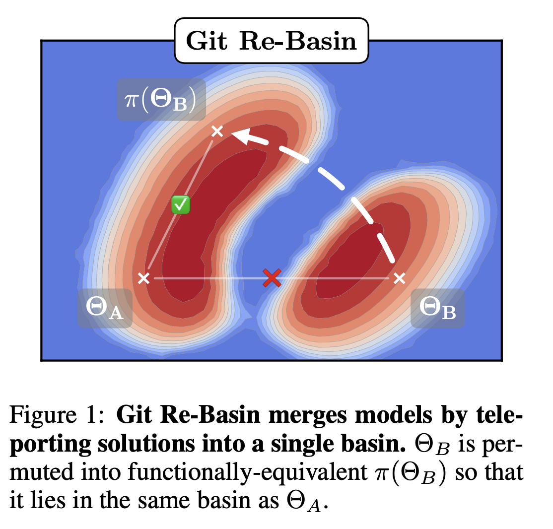
Ainsworth, Hayase, and Srinivasa [2] find that, after correcting for permutation symmetries, different weights are connected by a close-to-zero loss barrier linear mode connection. In other words, you can linearly interpolate between the permutation-corrected weights, and every point in the linearly interpolation has essentially the same loss. They conjecture that there is only global basin after correcting for these symmetries.

In general, correcting for these symmetries is NP-hard, so the argument of these authors depends on several approximate schemes to correct for the permutations [2].

![400](/media/pasted-image-20221220152152.png)

Universal Circuits

Some of the most compelling evidence for the low path-dependence world comes from the circuits-style research of Olah and collaborators. Across a range of computer vision models (AlexNet, InceptionV1, VGG19, ResnetV2-50), the circuits thread [3] finds features common to all of them such as curve and high-low frequency detectors [4], branch specialization [5], and weight banding [6]. More recently, the transformer circuits thread [7] has found universal features in language models, such as induction heads and bumps [8]. This is path independence at the highest level: regardless of architecture, hyperparameters, and initial weights different models learn the same things. In fact, low path-dependence ("universality") is often taken as a starting point for research on transparency and interpretability [4].

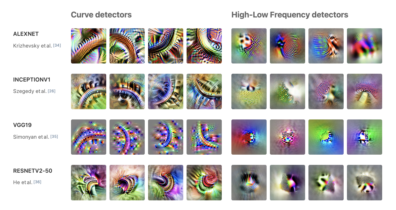
Universal circuits of computer vision models [4].

ML as Bayesian Inference

• $P_\beta(f)$ is the probability that $M$ expresses $f$ on $D$ upon a randomly sampled parametrization. This is our "prior"; it's what our network expresses on initialization.

• $V_\beta(f)$ is a volume with Gaussian measure that equals $P_\beta(f)$ under Gaussian sampling of network parameters.

  • This is a bit confusing. We're not talking about a continuous region of parameter space, but a bunch of variously distributed points and lower-dimensional manifolds. Mingard never explicitly points out why we expect a contiguous volume. That or maybe it's not necessary for it to be contiguous

• $\beta$ denotes the "Bayesian prior"

• $P_\text{opt}(f|S)$ is the probability of finding $f$ on $E$ under a stochastic optimizer like SGD trained to 100% accuracy on $S$.

• $P_\beta(f|S) = \frac{P(S|f) P_\beta(f)}{P_\beta(S)},$ is the probability of finding $f$ on $E$ upon randomly sampling parameters from i.i.d. Gaussians to get 100% accuracy on $S$.

  • This is what Mingard et al. call "Bayesian inference"
  • $P(S|f)=1$ if $f$ is consistent with $S$ and $0$ otherwise

• Double descent & Grokking

• Mingard et al.'s work on NNs as Bayesian.

Evidence Of High Path Dependence

• Why Comparing Single Performance Scores Does Not Allow to Conclusions About Machine Learning Approaches (Reimers et al., 2018)
• Deep Reinforcement Learning Doesn’t Work Yet (Irpan, 2018)
• Lottery Ticket Hypothesis

BERTS of a feather do not generalize together

Footnotes

1. This breaks down in the presence of regularization if two subsequent layers have different widths. ↩

2. For a given set of weights which sum to $0$, you can flip the signs of each of the weights, and the sum stays $0$. ↩

3. The claim of singular learning theory is that this non-injectivity is fundamental to the ability of neural networks to generalize. Roughly speaking, "simple" models that generalize better take up more volume in weight space, which make them easier to find. ↩