Context: We want to learn an appropriate function $f$ provided samples from a dataset $D_n = \{(X, Y)\}^n$.

Turns out, you can do better than the naive Bayes update,

Tempered Bayes

Introduce an inverse temperature, $\beta$, to get the tempered Bayes update [1]:

At first glance, this looks unphysical. Surely $P(A|B)^{\beta}\ P(B) = P(A, B)$ only when $\beta=1$?

If you're one for handwaving, you might just accept that this is just a convenient way to vary between putting more weight on the prior and more weight on the data. In any case, the tempered posterior is proper (integrable to one), as long as the untempered posterior is [2].

If you're feeling more thorough, think about the information. Introducing an inverse temperature is simply scaling the number of bits contained in the distribution. $P(X, Y|f) = \exp\{-\beta I(X, Y|f)\}$.

TODO: Check out Grünwald's Safe Bayes papers

Generalized Bayes

If you're feeling even bolder, you might replace the likelihood with a general loss term, $\ell_{\beta, n}(f)$, which measures performance on your dataset $D_n$,

where we write the normalizing constant or partition function as $Z_n$ to emphasize that it isn't really an "evidence" anymore.

The most natural choice for $\ell_{\beta,n}$ is the Gibbs measure:

where $r_n$ is the empirical risk of classical machine learning. You can turn any function into a probability.

Jeffreys Updates

TODO

Machine learning has gotten sloppy over the years.

It used to be that we thought carefully about the theoretical underpinnings of our models and proceeded accordingly.

We used the L2 loss in regression because, when doing maximum likelihood estimation over, L2 loss follows from the assumption that our samples are distributed according to i.i.d. Gaussian noise around some underlying deterministic function, $f_w$. If we have a likelihood defined as

where $w$ are the weights parametrizing our model.

We'd squeeze in some weight decay because when performing maximum a posteriori estimation it was equivalent to having a Gaussian prior over our weights, $\varphi(w)\sim \mathcal N(0, \lambda^{-1})$. For the same likelihood as above,

Nowadays, you just choose a loss function and twiddle with the settings until it works. Granted, this shift away from Bayesian-grounded techniques has given us a lot of flexibility. And it actually works (unlike much of the Bayesian project which turns out to just be disgustingly intractable).

But when you're a theorist trying to catch up to the empirical results, it turns out the Bayesian frame is rather useful. So we want a principled way of recovering probability distributions from arbitrary choices of loss function. Fortunately, this is possible.

The trick is simple: multiply your loss, $r_n(w)$, by some parameter $\beta$, whose units are such that $\beta\, r_n(w)$ is measured in bits. Now, negate and exponentiate and out pop a set of probabilities:

We put a probability distribution over the function space we want to model, and we can extract probabilities over outputs for given inputs.

So I was thinking about the dynamics of training, and looking for a way to model some phenomenon I had observed.

Initially, I had dismissed Brownian motion/random walk as an option because the trend was clearly linear — not square root. But then I was asked what Brownian motion looked like in higher dimensions and I panicked.

I had assumed that Brownian motion was universal — that dimensionality didn't enter into the equation (for average distance from the origin as a function of time). But now I was doubting myself.

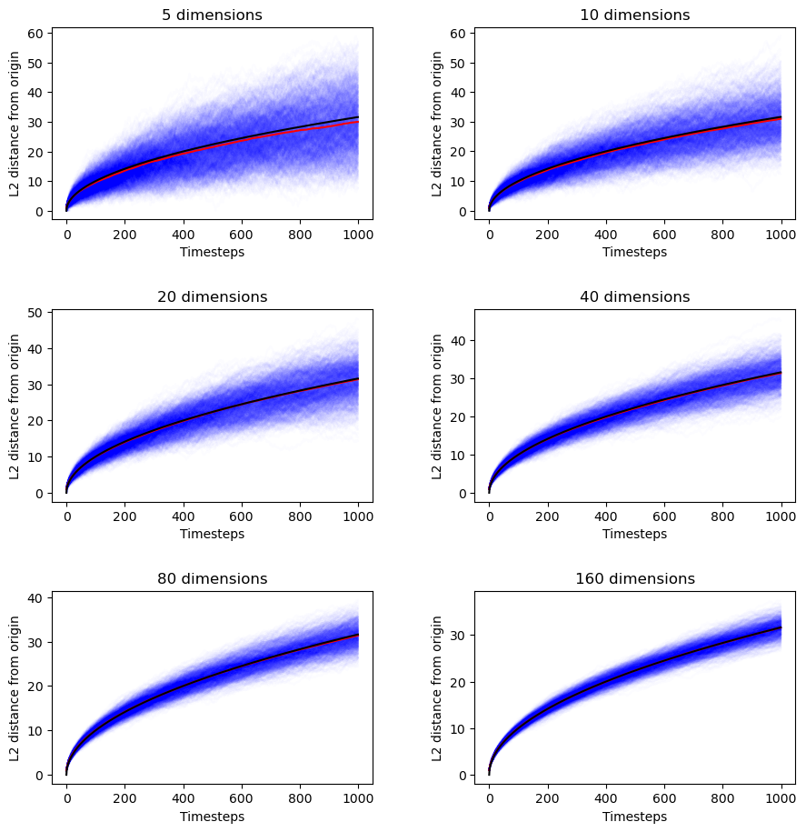
So I did a quick derivation, which I'm sharing because it gave me a new way to interpret the chi-squared distribution. Here's the set-up: we have a walker on a $D$-dimensional (square) lattice. At every timestep, the walker chooses uniformly among the $2D$ available directions to take one step.

This means that every dimension is sampled on average once every $D$ timesteps, so we can treat a $D$-dimensional walker after $N$ timesteps as a collection of $D$ independent $1$-dimensional walkers after $N/D$ timesteps.

If the $1$-dimensional walker's probability distribution is just a Gaussian centered at $0$ with standard deviation $\sqrt N$, then the probability for the $D$-dimensional walker is the product of $D$ univariate gaussians centered at $0$ with standard deviation $\sqrt{{N}/{D}}$.

But that means that the expected distance traveled by the $D$-dimensional walker, $\sqrt{\mathbb E[|\vec X|^2]}$, is just the square root of the chi-squared distribution,

scaled by a factor $\sqrt{N/D}$. (This is not the chi distribution, which we'd want if we were taking the square root before the expectation.)

In this context, $D$ is the number of degrees of freedom. After multiplying the mean of the chi distribution by our factor $\sqrt{N/D}$, we get

It's independent of lattice dimensionality. Just as I originally thought before starting to doubt myself before going down this rabbit hole before reestablishing my confidence.

If that's not enough for you, here are the empirical results.

def random_hyperwalk(n_dims: int, n_samples: int = 1_000, n_timesteps: int = 10_000) -> np.ndarray:
    state = np.zeros((n_samples, n_dims))
    distances = np.zeros((n_samples, n_timesteps))

    for t in tqdm(range(n_timesteps)):
        step = np.random.choice(np.arange(n_dims), n_samples)
        # print(step)
        directions = np.random.choice([-1, 1], n_samples)
        # print(directions)

        # TODO: vectorize this
        for i in range(n_samples):
            state[i, step[i]] += directions[i]

        # print(step, directions, state[:, step])
        distances[:, t] = np.linalg.norm(state, axis=1)

    return distances

def random_hyperwalk_scaling(n_dim_range: List[int], n_samples: int = 1_000, n_timesteps: int = 10_000):
    timesteps = np.arange(n_timesteps)
    predictions = np.sqrt(timesteps)
    trajectories = np.zeros((len(n_dim_range), n_samples, n_timesteps))

    fig, ax = plt.subplots(len(n_dim_range) // 2, 2, figsize=(10, 10))
    fig.tight_layout(pad=5.0)

    for I, n_dims in enumerate(n_dim_range):
        i, j = I // 2, I % 2

        trajectories[I, :, :] = random_hyperwalk(n_dims, n_samples, n_timesteps)
        mean_distances = np.mean(trajectories[I, :, :], axis=0)

        for k in range(n_samples):
            ax[i][j].plot(timesteps, trajectories[I, k, :], color="blue", alpha=0.01)
    
        ax[i][j].set_title(f"{n_dims} dimensions")
        ax[i][j].plot(timesteps, mean_distances, color="red")
        ax[i][j].plot(timesteps, predictions, color="black")
        ax[i][j].set_xlabel("Timesteps")
        ax[i][j].set_ylabel("L2 distance from origin")

    plt.show()


random_hyperwalk_scaling([5, 10, 20, 40, 80, 160], n_samples=1000, n_timesteps=1000)

Yesterday, I stumbled across the following question:

Does the following sum converge if you exclude all terms that don't include a $9$?

A little dash of anthropic reasoning suggests yes. Why would anyone have written the question on a poster and fixed it to the wall if otherwise? The base rate for chaotic trolls who also like math puzzles seems pretty low.

Fortunately, we can do better than anthropic reasoning, and, after thinking about it for a bit with Matt MacDermott, we found the answer:

First, let's rewrite the sum as

where $I_n$ is an indicator function,

The trick is to convert this sum over numbers into a sum over numbers of digits, then find an upper bound:

where $N_{d}$ is the number of numbers with $d$ digits that don't contain $9$, which we can compute by straightforward combinatorics,

So we end up with a new infinite sum for an upper bound to our original sum:

which converges.

Outline

• NTK

7. Recent progress in the theory of neural networks (MacAulay, 2019) (20 mins)
   • In the infinite-width limit:
     • Neal 1994: With Gaussian-distributed weights NNs limit to Gaussian process.
     • Novak 2018: Extension to CNNs
     • Yang 2019: And other NNs
     • Infinity-width limit -> Neural Tangent Kernel (like the first-order Taylor expansion of a NN about its initial parameters)
     • "The works above on the infinite-width limit explain, to some extent, the success of SGD at optimizing neural nets, because of the approximately linear nature of their parameter-space."
     • PAC-Bayes bounds. Binarized MNIST, Link with compression, and more. Bounds as a way of testing your theories

• Influence functions (sensitivity to a change in training examples) & Adversarial training examples[1]
  • We’re interested in how the optimal solution depends on $\theta$, so we define $w_* = r(\theta)$ to emphasize the functional dependency. The function $r(\theta)$ is called the response function, or rational reaction function, and the Implicit Function Theorem (IFT)
• Low path dependence: that one paper that adds adversarial noise, trains on it, then removes the adversarial noise (see Distill thread).

How much do the models we train depend on the paths they follow through weight space?

Should we expect to always get the same models for a given choice of hyperparameters and dataset? Or do the outcomes depend highly on quirks of the training process, such as the weight initialization and batch schedule?

If models are highly path-dependent, it could make alignment harder: we'd have to keep a closer eye on our models during training for chance forays into deception. Or it could make alignment easier: if alignment is unlikely by default, then increasing the variance in outcomes increases our odds of success.

Vivek Hebbar and Evan Hubinger have already explored the implications of path-dependence for alignment here. In this post, I'd like to take a step back and survey the machine learning literature on path dependence in current models. In future posts, I'll present a formalization of Hebbar and Hubinger's definition of "path dependence" that will let us start running experiments.

Evidence Of Low Path Dependence

Symmetries of Neural Networks

At a glance, neural networks appear to be rather path-dependent. Train the same network twice from a different initial state or with a different choice of hyperparameters, and the final weights will end up looking very different.

But weight space doesn't tell us everything. Neural networks are full of internal symmetries that allow a given function to be implemented by different choices of weights.

For example, you can permute two columns in one layer, and as long as you permute the corresponding rows in the next layer, the overall computation is unaffected. Likewise, with ReLU networks, you can scale up the inputs to a layer as long as you scale the outputs accordingly, i.e.,

$\text{ReLU}(x) = \alpha\, \text{ReLU}\left(\frac{x}{\alpha}\right),$

for any $\alpha > 0$¹. There are also a handful of "non-generic" symmetries, which the model is free to build or break during training. These correspond to, for example, flipping the orientations of the activation boundaries² or interpolating between two degenerate neurons that have the same ingoing weights.

Formally, if we treat a neural network as a mapping $f: \mathcal X \times \mathcal W \to \mathcal Y$, parametrized by weights $\mathcal W$, these internal symmetries mean that the mapping $\mathcal W \ni w \mapsto f_{w} \in \mathcal F$ is non-injective, where $f_{w}(x):=f(x, w)$.³

What we really care about is measuring similarity in $\mathcal F$. Unfortunately, this is an infinite-dimensional space, so we can't fully resolve where we are on any finite set of samples. So we have a trade-off: we can either perform our measurements in $\mathcal W$, where we have full knowledge, but where fully correcting for symmetries is intractable, or we can perform our measurements in $\mathcal F$, where we lack full knowledge, but

Correcting for Symmetries

Permutation-adjusted Symmetries

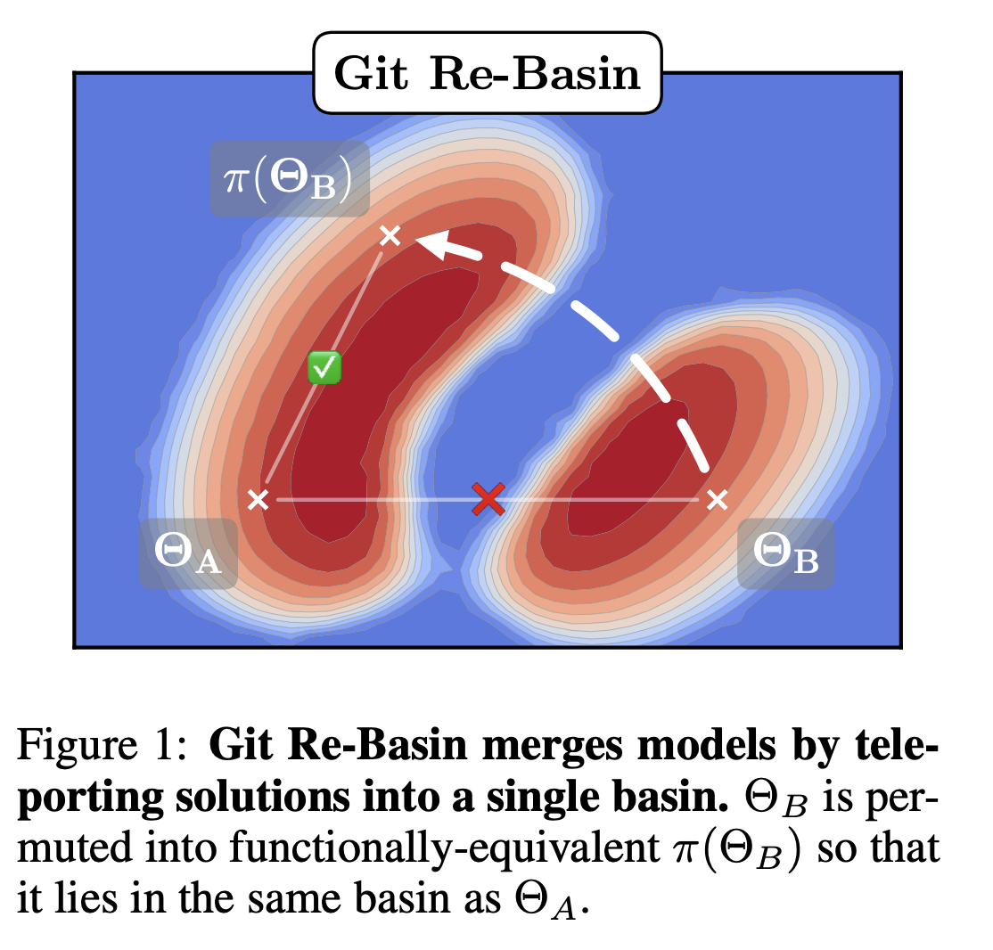
Ainsworth, Hayase, and Srinivasa [2] find that, after correcting for permutation symmetries, different weights are connected by a close-to-zero loss barrier linear mode connection. In other words, you can linearly interpolate between the permutation-corrected weights, and every point in the linearly interpolation has essentially the same loss. They conjecture that there is only global basin after correcting for these symmetries.

In general, correcting for these symmetries is NP-hard, so the argument of these authors depends on several approximate schemes to correct for the permutations [2].

![400](/media/pasted-image-20221220152152.png)

Universal Circuits

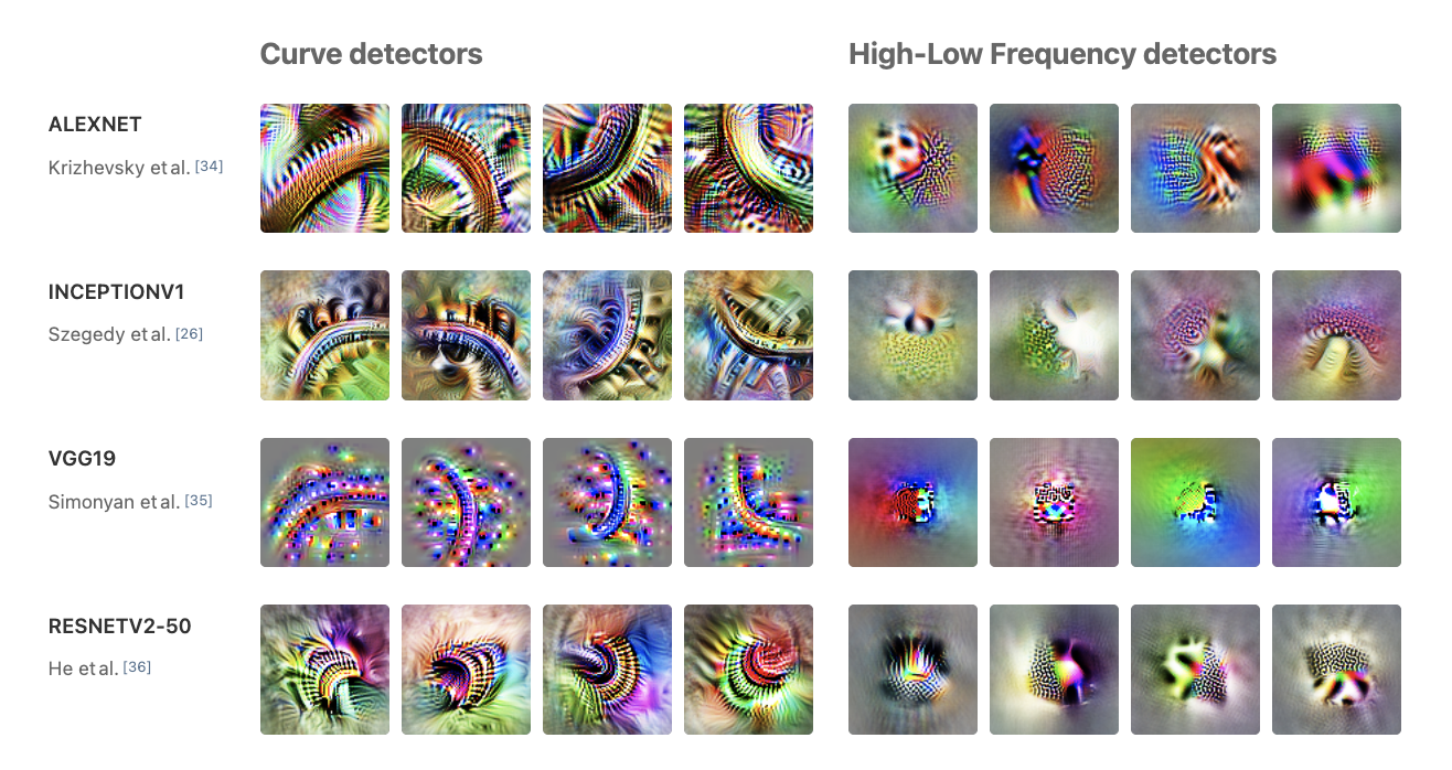
Some of the most compelling evidence for the low path-dependence world comes from the circuits-style research of Olah and collaborators. Across a range of computer vision models (AlexNet, InceptionV1, VGG19, ResnetV2-50), the circuits thread [3] finds features common to all of them such as curve and high-low frequency detectors [4], branch specialization [5], and weight banding [6]. More recently, the transformer circuits thread [7] has found universal features in language models, such as induction heads and bumps [8]. This is path independence at the highest level: regardless of architecture, hyperparameters, and initial weights different models learn the same things. In fact, low path-dependence ("universality") is often taken as a starting point for research on transparency and interpretability [4].

Universal circuits of computer vision models [4].

ML as Bayesian Inference

• $P_\beta(f)$ is the probability that $M$ expresses $f$ on $D$ upon a randomly sampled parametrization. This is our "prior"; it's what our network expresses on initialization.

• $V_\beta(f)$ is a volume with Gaussian measure that equals $P_\beta(f)$ under Gaussian sampling of network parameters.

  • This is a bit confusing. We're not talking about a continuous region of parameter space, but a bunch of variously distributed points and lower-dimensional manifolds. Mingard never explicitly points out why we expect a contiguous volume. That or maybe it's not necessary for it to be contiguous

• $\beta$ denotes the "Bayesian prior"

• $P_\text{opt}(f|S)$ is the probability of finding $f$ on $E$ under a stochastic optimizer like SGD trained to 100% accuracy on $S$.

• $P_\beta(f|S) = \frac{P(S|f) P_\beta(f)}{P_\beta(S)},$ is the probability of finding $f$ on $E$ upon randomly sampling parameters from i.i.d. Gaussians to get 100% accuracy on $S$.

  • This is what Mingard et al. call "Bayesian inference"
  • $P(S|f)=1$ if $f$ is consistent with $S$ and $0$ otherwise

• Double descent & Grokking

• Mingard et al.'s work on NNs as Bayesian.

Evidence Of High Path Dependence

• Why Comparing Single Performance Scores Does Not Allow to Conclusions About Machine Learning Approaches (Reimers et al., 2018)
• Deep Reinforcement Learning Doesn’t Work Yet (Irpan, 2018)
• Lottery Ticket Hypothesis

BERTS of a feather do not generalize together